Noise Resilience of an RGNG-based Grid Cell Model
Jochen Kerdels and Gabriele Peters
University of Hagen, Universit
¨
atsstrasse 1, D-58097 Hagen, Germany
Keywords:
Noise Resilience, Grid Cell Model, Input Space Representation, Recursive Growing Neural Gas.
Abstract:
Grid cells are neurons in the entorhinal cortex of mammals that are known for their peculiar, grid-like firing
patterns. We developed a generic computational model that describes the behavior of neurons with such firing
patterns in terms of a competitive, self-organized learning process. Here we investigate how this process can
cope with increasing amounts of noise in its input signal. We demonstrate, that the firing patterns of simulated
neurons are mostly unaffected with regard to their structure even if high levels of noise are present in the input.
In contrast, the maximum activity of the corresponding neurons decreases significantly with increasing levels
of noise. Based on these results we predict that real grid cells can retain their triangular firing patterns in the
presence of noise, but may exhibit a noticeable decrease in their peak firing rates.
1 INTRODUCTION
Several regions of the mammalian brain contain
neurons that exhibit peculiar, grid-like firing pat-
terns (Fyhn et al., 2004; Hafting et al., 2005; Boccara
et al., 2010; Killian et al., 2012; Yartsev et al., 2011;
Domnisoru et al., 2013; Jacobs et al., 2013). The most
common example for such neurons are so-called grid
cells found in the medial entorhinal cortex (MEC) of
rat (Fyhn et al., 2004; Hafting et al., 2005). The activ-
ity of these cells correlates with the animal’s location
in a periodic, triangular pattern that spans across the
entire environment of the animal.
We developed a generic computational model that
is able to describe the behavior of neurons with such
grid-like firing patterns (Kerdels and Peters, 2013;
Kerdels and Peters, 2015b; Kerdels, 2016). Here we
investigate how this model reacts to random noise in
its input signal as it would be expected to occur in
natural neurobiological circuits where each neuron re-
ceives input from hundreds to thousands of other neu-
rons (Koch, 2004)
1
.
The next section summarizes our grid cell model
briefly and highlights those mechanisms of the model
that are especially relevant to the investigation of
input signal noise. Subsequently, section 3 outlines
how scalable amounts of noise are added to the input
signal of our grid cell model. Section 4 then reports
and analyses the results obtained from simulation runs
1
p. 411ff
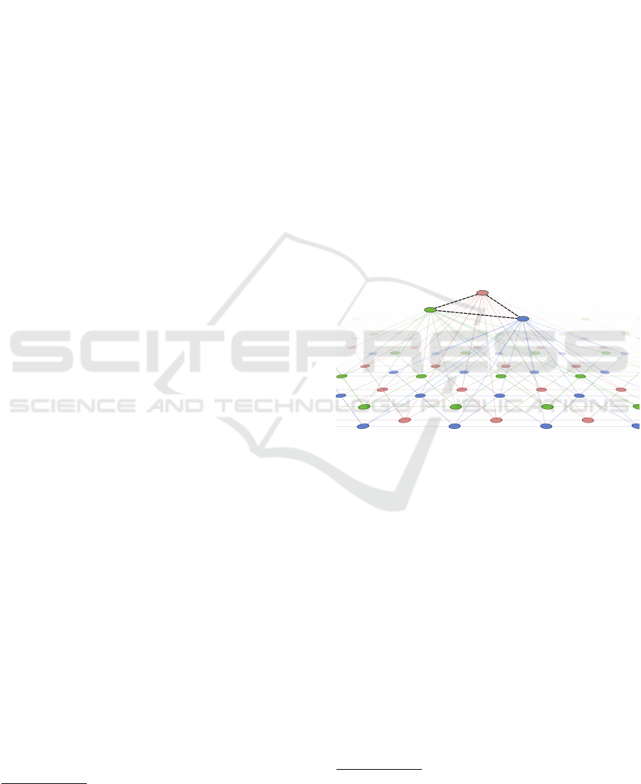
Figure 1: Illustration of the RGNG-based neuron model.
The top layer is represented by three units (red, green, blue)
connected by dashed edges. The prototypes of the top layer
units are themselves RGNGs. The units of these RGNGs
are illustrated in the second layer by corresponding colors.
with varying levels of noise. Finally, we discuss our
findings in section 5.
2 GRID CELL MODEL
We developed a generic neuron model that is able
to describe, among others, the behavior of grid
cells (Kerdels, 2016). At its core the model uses
the recursive growing neural gas (RGNG) algorithm
to describe the collective behavior of a group of
neurons. The RGNG algorithm extends the regu-
lar growing neural gas (GNG) algorithm proposed by
Fritzke (Fritzke, 1995) in a recursive fashion
2
. A reg-
2
A formal definition of the RGNG algorithm is provided
in the appendix.
Kerdels, J. and Peters, G.
Noise Resilience of an RGNG-based Grid Cell Model.
DOI: 10.5220/0006045400330041
In Proceedings of the 8th International Joint Conference on Computational Intelligence (IJCCI 2016) - Volume 3: NCTA, pages 33-41
ISBN: 978-989-758-201-1
Copyright
c
 2016 by SCITEPRESS – Science and Technology Publications, Lda. All rights reserved
33

ular GNG is an unsupervised learning algorithm that
approximates the structure of its input space with a
network of units where each unit represents a local
region of input space while the network itself repre-
sents the input space topology. In a recursive GNG
or RGNG the units can not only represent local input
space regions but may also represent entire RGNGs
themselves resulting in a layered, hierarchical struc-
ture of interleaved input space representations.
In our grid cell model we use a single RGNG with
two layers to model a group of neurons (Fig. 1). The
units in the top layer (TL) represent the individual
cells of the group. Each of these TL units contains an
RGNG located in the bottom layer (BL). These BL-
RGNGs can be interpreted as the dendritic trees of the
neurons, each of which learning a separate represen-
tation of the entire input space. The units of the BL-
RGNGs correspond to local subsections of the den-
dritic tree that recognize input patterns from specific,
local regions of input space. In the model, these local
regions are represented by so-called reference vectors
or prototypes. Thus, each modelled neuron (TL unit)
has a set of prototypes (BL units) that are arranged
in a network (BL RGNG) that constitutes a piece-
wise approximation of the neuron’s input space. The
neurons (TL units) themselves are organized in a net-
work (TL RGNG) as well resulting in an interleaved
arrangement of the individual input space approxima-
tions.
Please note that the term “neuron” is used differ-
ently here compared to its regular usage in a growing
neural gas context. It is used synonymously only with
the TL units of the model and not the BL units. Fur-
thermore, the RGNG is inherently different from ex-
isting hierarchical versions of the growing neural gas
like those proposed by, e.g., Doherty et al. (Doherty
et al., 2005) or Podolak and Bartocha (Podolak and
Bartocha, 2009). These approaches represent the in-
put space in a hierarchical fashion with every unit of
the hierarchical GNG corresponding to a single local
region of input space. In our model, this holds true
only for the BL units whereas every TL unit repre-
sents the entire input space.
2.1 Learning
The two-layer RGNG used in the grid cell model has
no explicit training phase and updates its input space
approximation continuously. In a first step, each in-
put ξ is processed by all neurons. To this end every
neuron determines the best and second best matching
units (BMUs) termed s
1
and s
2
, respectively. Units
s
1
and s
2
are those BL units whose prototypes s
1
w
and s
2
w are closest to the input ξ according to a dis-
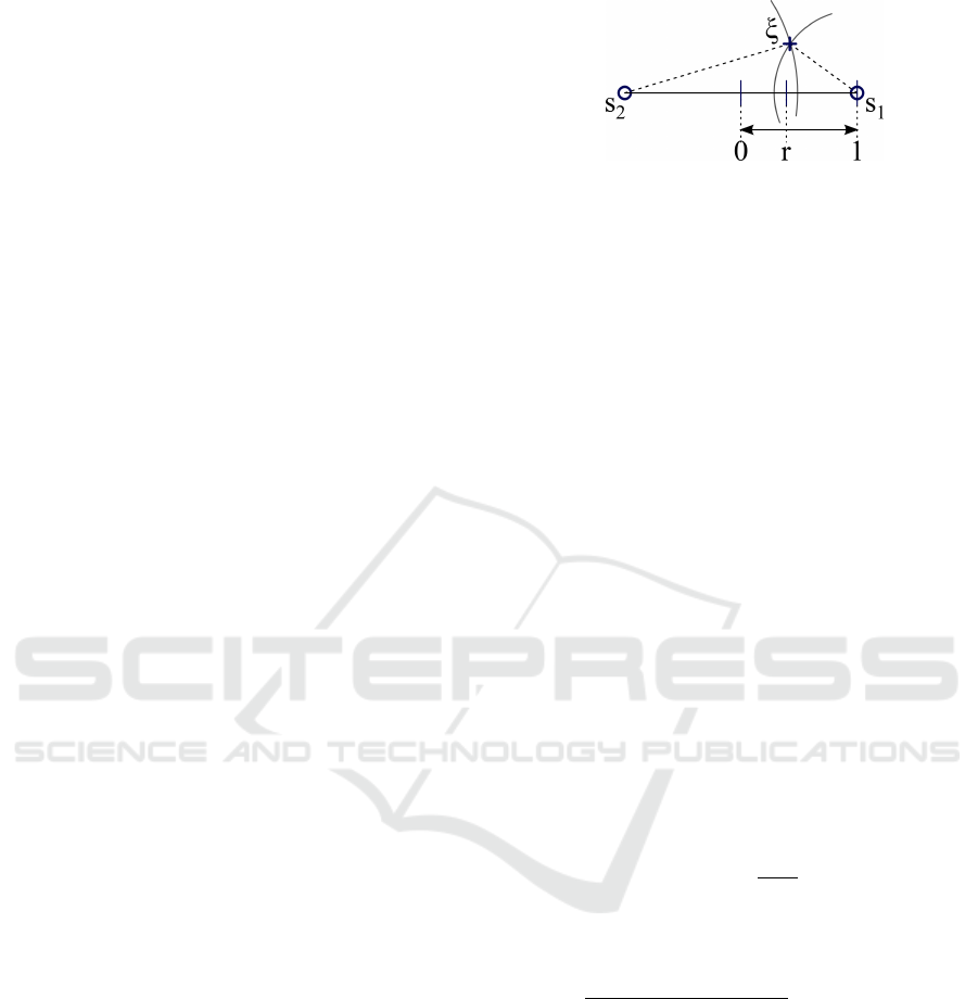
Figure 2: Geometric interpretation of ratio r, which is used
as basis for an approximation of the top layer unit’s “activ-
ity”.
tance function D. Once determined, the BMUs of ev-
ery neuron are adapted towards the input ξ and the
corresponding BL networks are updated where nec-
essary.
In a second step, the single neuron whose BMU
was closest to the input and its direct neighboring neu-
rons in the TL network are allowed to adapt towards
the input a second time. This selective adaptation
aligns the input space representations of the individ-
ual neurons and interleaves them evenly to cover the
input space as well as possible (Kerdels, 2016).
2.2 Activity Approximation
The RGNG-based model describes a group of neu-
rons for which we would like to derive their “activ-
ity” for any given input as a scalar that represents
the momentary firing rate of the particular neuron.
Yet, the RGNG algorithm itself does not provide a
direct measure that could be used to this end. There-
fore, we derive the activity a
u
of a modelled neuron u
based on the neuron’s best and second best matching
BL units s
1
and s
2
with respect to a given input ξ as:
a
u
:= e
−
(1−r)
2
2σ
2
,
with σ = 0.2 and ratio r:
r :=
D(s
2
w, ξ) − D(s
1
w, ξ)
D(s
1
w, s
2
w)
, s
1
, s
2
∈ uwU,
using a distance function D. Figure 2 provides a geo-
metric interpretation of the ratio r. If input ξ is close
to BMU s
1
in relation to s
2
, ratio r becomes 1. If on
the other hand input ξ has about the same distance
to s
1
as it has to s
2
, ratio r becomes 0.
This measure of activity allows to correlate the re-
sponse of a neuron to a given input with further vari-
ables. An example of such a correlation is shown
in figure 3b as a firing rate map, which correlates
the animal’s location (Fig. 3a) with the activity of a
simulated grid cell at that location. The firing rate
maps resulting from our simulations are constructed
NCTA 2016 - 8th International Conference on Neural Computation Theory and Applications
34

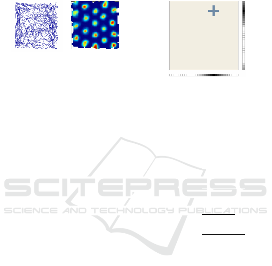
(a) (b)
Figure 3: (a) Example trace of rat movement within a
rectangular, 1 m × 1m environment recorded for a duration
of 10 minutes. Movement data published by Sargolini et
al. (Sargolini et al., 2006). (b) Color-coded firing rate map
of a simulated grid cell ranging from dark blue (no activity)
to red (maximum activity).
according to the procedures described by Sargolini et
al. (Sargolini et al., 2006) but using a 5 × 5 boxcar
filter for smoothing instead of a Gaussian kernel as
introduced by Stensola et al. (Stensola et al., 2012).
This conforms to the de facto standard of rate map
construction in the grid cell literature. Each rate map
integrates position and activity data over 30000 time
steps corresponding to a single experimental trial with
a duration of 10 minutes recorded at 50Hz.
3 INPUT SIGNAL
In general, the RGNG-based neuron model is inde-
pendent of any specific type of input space and can
process arbitrary input signals. However, only in-
put spaces with certain characteristics will cause the
modelled neurons to exhibit grid-like firing patterns
with respect to a given variable, e.g., the animal’s lo-
cation. More precisely, grid-like firing patterns will
only emerge if the input signals originate from a uni-
formly distributed, two-dimensional manifold in the
input space that correlates with the respective exter-
nal variable.
In the case of grid cells there are many conceivable
input spaces that meet these requirements (Kerdels,
2016). For our experiments we choose an input space
where the position of the animal is encoded by two
vectors as shown in figure 4. The two-dimensional
position is represented by the activity of two sets of
cells that each are connected in a one-dimensional,
periodic fashion like, e.g., a one-dimensional ring at-
tractor network. Similar types of input signals for grid
cell models were proposed in the literature by, e.g.,
Mhatre et al. (Mhatre et al., 2010) as well as Pilly and
Grossberg (Pilly and Grossberg, 2012).
For the experiments discussed below the input sig-
nal ξ := (v
x
, v
y
) is implemented as two concatenated
50-dimensional vectors v
x
and v
y
. To generate an in-
Figure 4: The input signal for our experiments is derived
by encoding a position (blue cross) in a periodic, two-
dimensional input space (square) as the activity (black =
high, white = low) of two sets of cells (vertical and hori-
zontal groups of small boxes) that each are connected in a
one-dimensional, periodic fashion, i.e., the activity wraps
around at the borders of the resulting vectors.
put signal a position (x, y) ∈ [0, 1]× [0, 1] is read from
traces (Fig. 3a) of recorded rat movements that were
published by (Sargolini et al., 2006) and mapped onto
the corresponding elements of v
x
and v
y
as follows:
v
x
i
:= max

1 −




i − bdx + 0.5c
s




,
1 −




d + i − bdx + 0.5c
s




, 0

,
v
y
i
:= max

1 −




i − bdy + 0.5c
s




,
1 −




d + i − bdy + 0.5c
s




, 0

,
∀i ∈
{
0. . . d − 1
}
,
with d = 50 and s = 8. The parameter s controls the
slope of the activity peak with higher values of s re-
sulting in a broader peak.
Each input vector ξ := ( ˜v
x
, ˜v
y
) was then aug-
mented by noise as follows:
˜v
x
i
:= max[ min[ v
x
i
+ ξ
n
(2U
rnd
− 1), 1] , 0] ,
˜v
y
i
:= max

min

v
y
i
+ ξ
n
(2U
rnd
− 1), 1

, 0

,
∀i ∈
{
0. . . d − 1
}
,
with maximum noise level ξ
n
and uniform random
values U
rnd
∈ [0, 1]. The rationale for this noise model
is as follows. Each element of the input vector rep-
Noise Resilience of an RGNG-based Grid Cell Model
35

resents the normalized firing rate of an input neu-
ron, where typical peak firing rates of neurons in the
parahippocampal-hippocampal region range between
1Hz and 50Hz (Hafting et al., 2005; Sargolini et al.,
2006; Boccara et al., 2010; Krupic et al., 2012). Some
proportion of this firing rate is due to spontaneous
activity of the corresponding neuron. According to
Koch (Koch, 2004) this random activity can occur
about once per second, i.e., at 1Hz. Hence, the pro-
portion of noise in the normalized firing rate result-
ing from this spontaneous firing can be expected to
lie between 1.0 and 0.02 given the peak firing rates
stated above. As we have no empirical data on the
distribution of peak firing rates in the input signal of
grid cells we assume a uniform distribution. The pa-
rameter ξ
n
allows to control the maximum noise level
or the assumed minimal peak firing rate (implicitly).
For example, a maximum noise level of ξ
n
= 0.1 cor-
responds to a minimal peak firing rate of 10Hz, and a
level of ξ
n
= 0.5 corresponds to a minimal peak firing
rate of 2Hz.
4 SIMULATION RESULTS
To investigate how the RGNG-based grid cell model
reacts to noise in its input signal we ran a series of
simulations with increasing levels ξ
n
of noise (or, cor-
respondingly, decreasing minimal peak firing rates).
All simulation runs used the fixed set of parame-
ters shown in table 1 (appendix). Both, the num-
ber θ
1
M = 100 of simulated grid cells as well as
the number θ
2
M = 20 of dendritic subsections per
cell are chosen to lie within a biologically plausible
range. The latter number can be estimated based on
the morphological properties of MEC layer II stellate
cells, which are presumed to be one type of princi-
pal neurons that exhibit grid-like firing patterns (Gio-
como et al., 2007; Giocomo and Hasselmo, 2008).
The dendritic tree of these neurons has about 7500
to 15000 spines, each hosting one or more synaptic
connections (Lingenhhl and Finch, 1991). In our ex-
periments we assume that the input space of each grid
cell is comprised by the output of 100 input neurons
and that each grid cell recognizes θ
2
M = 20 differ-
ent input patterns originating from that space. This
parametrization results in 3.75 to 7.5 available spines
for each input dimension in a prototype pattern. This
is a conservative choice that provides some margin
for possible variability in input dimension and num-
ber of prototypes. Estimating the number θ
1
M of
grid cells in a grid cell group
3
is more difficult. Sten-
3
Grid cells are organized in groups that share the same
grid spacing and grid orientation (Stensola et al., 2012).
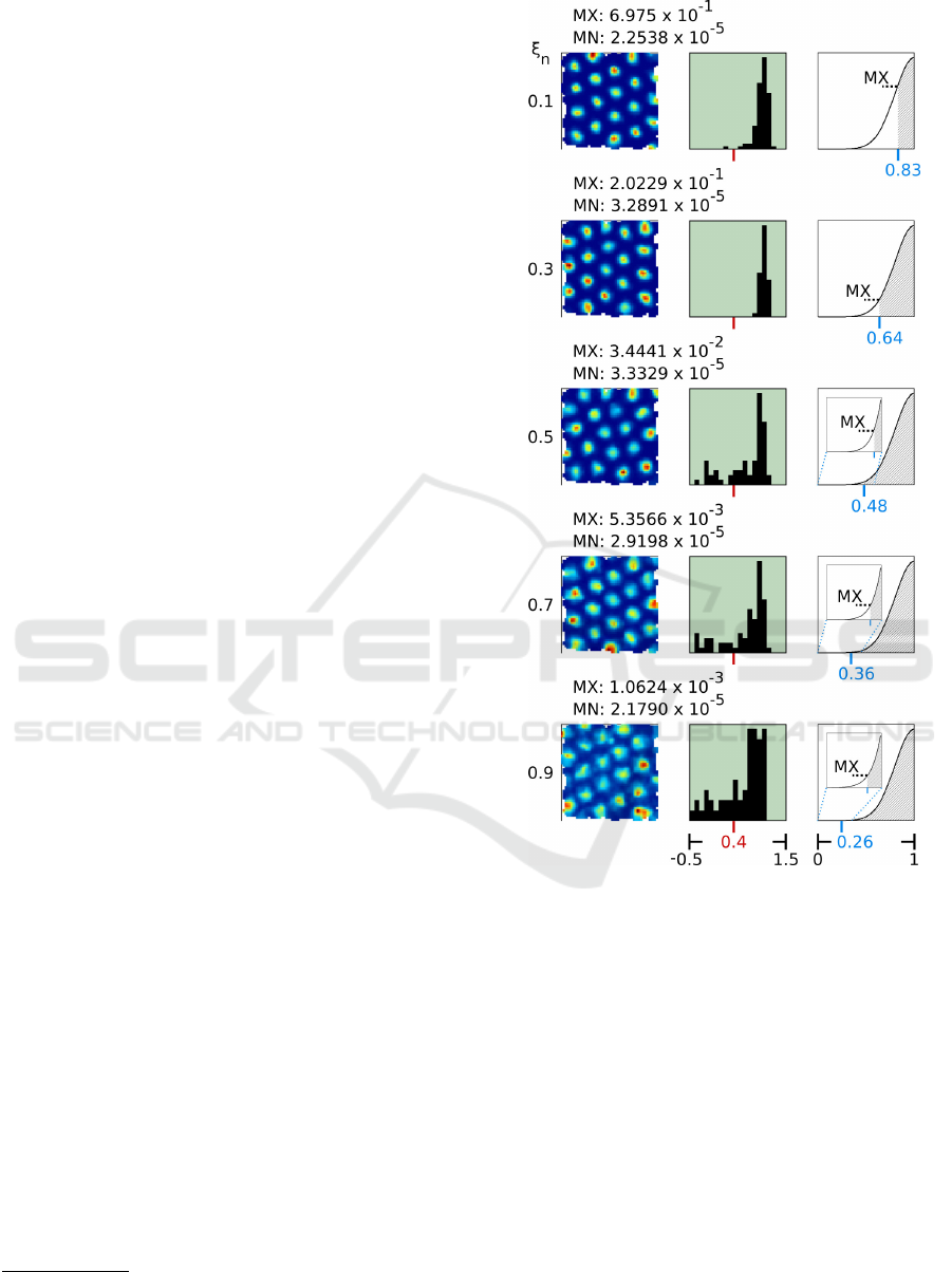
Figure 5: Artificial rate maps (left), gridness distributions
(middle), and activity function plots (right) of simulation
runs with varying levels ξ
n
of noise (rows) added to the
inputs. All simulation runs used a fixed set of parameters
(Table 1) and processed location inputs derived from move-
ment data published by Sargolini et al. (Sargolini et al.,
2006). Each artificial rate map was chosen randomly from
the particular set of rate maps. Average maximum activity
(MX) and average minimum activity (MN) across all rate
maps stated above. Gridness threshold of 0.4 indicated by
red marks. Values of ratio r at average maximum activity
(MX) given in blue. Insets show magnified regions of the
activity function where MX values are low.
sola et al. (Stensola et al., 2012) estimate that there
are up to 10 different, discrete groups of grid spac-
ings present in the MEC. Thus, as an upper bound the
number of grid cells per grid cell group can be esti-
mated as one-tenth of the total number of grid cells
in layer II of the rat MEC. This number is not exactly
NCTA 2016 - 8th International Conference on Neural Computation Theory and Applications
36

known. Based on empirical data it can be estimated to
lie between 14200 (Gatome et al., 2010; Krupic et al.,
2012) and 25000 (Hafting et al., 2005; Sargolini et al.,
2006; Boccara et al., 2010) cells resulting in an up-
per bound for the size θ
1
M of a grid cell group to
lie between 1420 and 2500 grid cells. In contrast, a
lower bound for the group size can not be estimated
reliably as the actual number of observed grid cells
per grid cell group is quite small (< 50) in individual
animals (Stensola et al., 2012; Krupic et al., 2012).
Grid cell groups may be more numerous and contain
fewer cells than indicated by the upper bound. How-
ever, in the context of our RGNG-based model this
uncertainty appears to be noncritical. As reported by
Kerdels (Kerdels, 2016) the behavior of the simulated
grid cells is not influenced by the particular size of
the grid cell group in any significant way. Thus, we
chose a value of θ
1
M = 100 as a compromise be-
tween the possibility of a few large and many small
grid cell groups. For a full, detailed derivation and
characterization of the other parameters we refer to
Kerdels (Kerdels, 2016).
For the simulation runs reported here we used a se-
quence of input locations taken from recorded move-
ment data of rats running around in a square environ-
ment while chasing food pellets. To keep the simula-
tion runs comparable, each run used the same trajec-
tory. The data was published by Sargolini et al. (Sar-
golini et al., 2006) and is available for download
4
.
Figure 5 summarizes the results of these experi-
ments. For each run (rows) the figure shows the firing
rate map of one grid cell that was randomly chosen
from the simulated grid cell group, the distribution
of gridness scores
5
of all simulated cells, and an ac-
tivity function plot indicating the maximum activity
exhibited by any of the simulated grid cells. The ex-
emplary rate maps and gridness score distributions in-
dicate that the RGNG-based model is able to tolerate
increasing levels ξ
n
∈
{
0.1, 0.3, 0.5, 0.7, 0.9
}
of noise
without loosing its ability to form the characteristic,
triangular firing patterns of grid cells. However, with
increasing noise level the maximum average activity
(MX) present in the rate maps drops by two orders of
magnitude. This decrease is clearly visible in the ac-
tivity function plots shown in the right column of fig-
ure 5. Yet, the minimal difference between the max-
imum average activity (MX) and the minimum aver-
age activity (MN) for any given noise level ξ
n
is at
least two orders of magnitude, i.e., each cell’s activity
may be normalized with respect to the particular noise
4
http://www.ntnu.edu/kavli/research/grid-cell-data
5
The gridness score ([−2, 2]) is a measure of how grid-
like the firing pattern of a neuron is. Neurons with gridness
scores greater 0.4 are commonly identified as grid cell.
level without much disturbance of the grid-like firing
pattern.
The reduction of the maximum average activity
with increasing noise levels can be explained by the
ratio r used to derive each cell’s activity (Fig. 2). The
ratio r describes the relative distance of the current
input ξ to the best matching unit s
1
and the second
best matching unit s
2
. If r is close to zero, the in-
put has roughly the same distance to unit s
1
and to
unit s
2
resulting in a low activity of the corresponding
neuron. If, on the other hand, r is close to one, the
input is close to the best matching unit s
1
yielding a
high activity of the simulated neuron. With increasing
noise the probability that an input matches the proto-
type of the best matching unit very closely decreases
substantially. Without noise all inputs originate from
a lower-dimensional manifold in input space. Adding
noise to these inputs moves the inputs away from this
manifold in random directions creating a local, high-
dimensional region surrounding the low-dimensional
manifold that is prone to effects that are commonly
referred to as the curse of dimensionality. As a conse-
quence, each BL prototype becomes surrounded with
a kind of “dead zone” for which it is unlikely that an
input will originate from it. These dead zones are in-
dicated in the right column of figure 5 as light gray
areas in the activity function plots. The values of the
ratio r at the border of these zones (blue marks in
Fig 5) define the probable maximum activity of the
corresponding neurons.
5 CONCLUSIONS
The simulation results presented here indicate that the
prototype-based representation of input space utilized
by our grid cell model shows a high resilience to noise
present in its input signal. This means, that even input
signals with very low peak firing rates around 1Hz
and a corresponding large proportion of noise through
spontaneous activity can be processed by our model.
According to these results, we would expect that real
grid cells
• can process inputs with low peak firing rates,
• may show a similar reduction in activity when the
proportion of noise in their inputs is high, and
• would not suffer a degradation of their firing field
geometry in such a case.
These hypothesis may be actively tested by experi-
ments that introduce controlled noise to the input sig-
nal, e.g., by the use of optogenetics (Hausser, 2014).
Alternatively, a passive comparison of the peak firing
rates present in the input signal of a grid cell and the
Noise Resilience of an RGNG-based Grid Cell Model
37

resulting peak firing rate of the grid cell itself may in-
dicate a possible correlation. To the best of our knowl-
edge no such experiments were done yet.
However, neurons are also known to have several
strategies to directly compensate for noise in their in-
put signal by, e.g., changing electrotonic properties
of their cell membranes (Koch, 2004). Such adapta-
tions could be represented in our grid cell model by
normalizing ratio r with respect to the level of noise.
How such a normalization could be implemented is
one subject of our future research.
In addition to these neurobiological aspects the
presented results also illustrate the general ability of
prototype-based learning algorithms like the GNG or
RGNG to learn the structure of an input space even in
the presence of very high levels of noise as shown in
the last row of figure 5.
REFERENCES
Boccara, C. N., Sargolini, F., Thoresen, V. H., Solstad, T.,
Witter, M. P., Moser, E. I., and Moser, M.-B. (2010).
Grid cells in pre- and parasubiculum. Nat Neurosci,
13(8):987–994.
Doherty, K., Adams, R., and Davey, N. (2005). Hierar-
chical growing neural gas. In Ribeiro, B., Albrecht,
R., Dobnikar, A., Pearson, D., and Steele, N., editors,
Adaptive and Natural Computing Algorithms, pages
140–143. Springer Vienna.
Domnisoru, C., Kinkhabwala, A. A., and Tank, D. W.
(2013). Membrane potential dynamics of grid cells.
Nature, 495(7440):199–204.
Fritzke, B. (1995). A growing neural gas network learns
topologies. In Advances in Neural Information Pro-
cessing Systems 7, pages 625–632. MIT Press.
Fyhn, M., Molden, S., Witter, M. P., Moser, E. I., and
Moser, M.-B. (2004). Spatial representation in the en-
torhinal cortex. Science, 305(5688):1258–1264.
Gatome, C., Slomianka, L., Lipp, H., and Amrein, I. (2010).
Number estimates of neuronal phenotypes in layer
{II} of the medial entorhinal cortex of rat and mouse.
Neuroscience, 170(1):156 – 165.
Giocomo, L. M. and Hasselmo, M. E. (2008). Time con-
stants of h current in layer ii stellate cells differ along
the dorsal to ventral axis of medial entorhinal cortex.
The Journal of Neuroscience, 28(38):9414–9425.
Giocomo, L. M., Zilli, E. A., Fransn, E., and Hasselmo,
M. E. (2007). Temporal frequency of subthreshold os-
cillations scales with entorhinal grid cell field spacing.
Science, 315(5819):1719–1722.
Hafting, T., Fyhn, M., Molden, S., Moser, M.-B., and
Moser, E. I. (2005). Microstructure of a spatial map
in the entorhinal cortex. Nature, 436(7052):801–806.
Hausser, M. (2014). Optogenetics: the age of light. Nat
Meth, 11(10):1012–1014.
Jacobs, J., Weidemann, C. T., Miller, J. F., Solway, A.,
Burke, J. F., Wei, X.-X., Suthana, N., Sperling, M. R.,
Sharan, A. D., Fried, I., and Kahana, M. J. (2013). Di-
rect recordings of grid-like neuronal activity in human
spatial navigation. Nat Neurosci, 16(9):1188–1190.
Kerdels, J. (2016). A Computational Model of Grid Cells
based on a Recursive Growing Neural Gas. PhD the-
sis, FernUniversit
¨
at in Hagen, Hagen.
Kerdels, J. and Peters, G. (2013). A computational model
of grid cells based on dendritic self-organized learn-
ing. In Proceedings of the International Conference
on Neural Computation Theory and Applications.
Kerdels, J. and Peters, G. (2015a). Analysis of high-
dimensional data using local input space histograms.
Neurocomputing, 169:272 – 280.
Kerdels, J. and Peters, G. (2015b). A new view on grid cells
beyond the cognitive map hypothesis. In 8th Confer-
ence on Artificial General Intelligence (AGI 2015).
Killian, N. J., Jutras, M. J., and Buffalo, E. A. (2012). A
map of visual space in the primate entorhinal cortex.
Nature, 491(7426):761–764.
Koch, C. (2004). Biophysics of Computation: Information
Processing in Single Neurons. Computational Neuro-
science Series. Oxford University Press, USA.
Krupic, J., Burgess, N., and OKeefe, J. (2012). Neural
representations of location composed of spatially pe-
riodic bands. Science, 337(6096):853–857.
Lingenhhl, K. and Finch, D. (1991). Morphological char-
acterization of rat entorhinal neurons in vivo: soma-
dendritic structure and axonal domains. Experimental
Brain Research, 84(1):57–74.
Mhatre, H., Gorchetchnikov, A., and Grossberg, S. (2010).
Grid cell hexagonal patterns formed by fast self-
organized learning within entorhinal cortex (published
online 2010). Hippocampus, 22(2):320–334.
Pilly, P. K. and Grossberg, S. (2012). How do spatial learn-
ing and memory occur in the brain? coordinated learn-
ing of entorhinal grid cells and hippocampal place
cells. J. Cognitive Neuroscience, pages 1031–1054.
Podolak, I. and Bartocha, K. (2009). A hierarchical
classifier with growing neural gas clustering. In
Kolehmainen, M., Toivanen, P., and Beliczynski, B.,
editors, Adaptive and Natural Computing Algorithms,
volume 5495 of Lecture Notes in Computer Science,
pages 283–292. Springer Berlin Heidelberg.
Sargolini, F., Fyhn, M., Hafting, T., McNaughton, B. L.,
Witter, M. P., Moser, M.-B., and Moser, E. I.
(2006). Conjunctive representation of position, di-
rection, and velocity in entorhinal cortex. Science,
312(5774):758–762.
Stensola, H., Stensola, T., Solstad, T., Froland, K., Moser,
M.-B., and Moser, E. I. (2012). The entorhinal grid
map is discretized. Nature, 492(7427):72–78.
Yartsev, M. M., Witter, M. P., and Ulanovsky, N. (2011).
Grid cells without theta oscillations in the entorhinal
cortex of bats. Nature, 479(7371):103–107.
NCTA 2016 - 8th International Conference on Neural Computation Theory and Applications
38

APPENDIX
Recursive Growing Neural Gas
The recursive growing neural gas (RGNG) has essen-
tially the same structure as the regular growing neural
gas (GNG) proposed by Fritzke (Fritzke, 1995). Like
a GNG an RGNG g can be described by a tuple
6
:
g := (U,C, θ) ∈ G,
with a set U of units, a set C of edges, and a set θ of
parameters. Each unit u is described by a tuple:
u := (w, e) ∈ U, w ∈ W := R
n
∪ G, e ∈ R,
with the prototype w, and the accumulated error e.
Note that in contrast to the regular GNG the proto-
type w of an RGNG unit can either be a n-dimensional
vector or another RGNG. Each edge c is described by
a tuple:
c := (V,t) ∈ C, V ⊆ U ∧ |V | = 2, t ∈ N,
with the units v ∈ V connected by the edge and the
age t of the edge. The direct neighborhood E
u
of a
unit u ∈ U is defined as:
E
u
:=
{
k|∃ (V,t) ∈ C, V =
{
u, k
}
, t ∈ N
}
.
The set θ of parameters consists of:
θ :=
{
ε
b
, ε
n
, ε
r
, λ, τ, α, β, M
}
.
Compared to the regular GNG the set of parameters
has grown by θε
r
and θM. The former parameter is
a third learning rate used in the adaptation function
A (see below). The latter parameter is the maximum
number of units in an RGNG. This number refers
only to the number of “direct” units in a particular
RGNG and does not include potential units present in
RGNGs that are prototypes of these direct units.
Like its structure the behavior of the RGNG is ba-
sically identical to that of a regular GNG. However,
since the prototypes of the units can either be vectors
or RGNGs themselves, the behavior is now defined
by four functions. The distance function
D(x, y) : W ×W → R
determines the distance either between two vectors,
two RGNGs, or a vector and an RGNG. The interpo-
lation function
I(x, y) : (R
n
× R
n
) ∪ (G × G) → W
generates a new vector or new RGNG by interpolat-
ing between two vectors or two RGNGs, respectively.
The adaptation function
A(x, ξ, r) : W × R
n
× R → W
6
The notation gα is used to reference the element α
within the tuple.
adapts either a vector or RGNG towards the input vec-
tor ξ by a given fraction r. Finally, the input function
F(g, ξ) : G × R
n
→ G × R
feeds an input vector ξ into the RGNG g and returns
the modified RGNG as well as the distance between ξ
and the best matching unit (BMU, see below) of g.
The input function F contains the core of the RGNG’s
behavior and utilizes the other three functions, but is
also used, in turn, by those functions introducing sev-
eral recursive paths to the program flow.
F(g, ξ): The input function F is a generalized ver-
sion of the original GNG algorithm that facilitates the
use of prototypes other than vectors. In particular, it
allows to use RGNGs themselves as prototypes result-
ing in a recursive structure. An input ξ ∈ R
n
to the
RGNG g is processed by the input function F as fol-
lows:
• Find the two units s
1
and s
2
with the smallest dis-
tance to the input ξ according to the distance func-
tion D:
s
1
:= argmin
u∈gU
D(uw, ξ),
s
2
:= argmin
u∈gU \
{
s
1
}
D(uw, ξ).
• Increment the age of all edges connected to s
1
:
∆ct = 1, c ∈ gC ∧ s
1
∈ cV .
• If no edge between s
1
and s
2
exists, create one:
gC ⇐ gC ∪
{
(
{
s
1
, s
2
}
, 0)
}
.
• Reset the age of the edge between s
1
and s
2
to
zero:
ct ⇐ 0, c ∈ gC ∧ s
1
, s
2
∈ cV .
• Add the squared distance between ξ and the pro-
totype of s
1
to the accumulated error of s
1
:
∆s
1
e = D(s
1
w, ξ)
2
.
• Adapt the prototype of s
1
and all prototypes of its
direct neighbors:
s
1
w ⇐ A(s
1
w, ξ, gθε
b
),
s
n
w ⇐ A(s
n
w, ξ, gθε
n
), ∀s
n
∈ E
s
1
.
• Remove all edges with an age above a given
threshold τ and remove all units that no longer
have any edges connected to them:
gC ⇐ gC \
{
c|c ∈ gC ∧ ct > gθτ
}
,
gU ⇐ gU \
{
u|u ∈ gU ∧ E
u
=
/
0
}
.
Noise Resilience of an RGNG-based Grid Cell Model
39

• If an integer-multiple of gθλ inputs was pre-
sented to the RGNG g and |gU| < gθM, add a
new unit u. The new unit is inserted “between” the
unit j with the largest accumulated error and the
unit k with the largest accumulated error among
the direct neighbors of j. Thus, the prototype uw
of the new unit is initialized as:
uw := I( jw, kw), j = argmax
l∈gU
(le) ,
k = argmax
l∈E
j
(le) .
The existing edge between units j and k is re-
moved and edges between units j and u as well
as units u and k are added:
gC ⇐ gC \
{
c|c ∈ gC ∧ j, k ∈ cV
}
,
gC ⇐ gC ∪
{
(
{
j, u
}
, 0), (
{
u, k
}
, 0)
}
.
The accumulated errors of units j and k are de-
creased and the accumulated error ue of the new
unit is set to the decreased accumulated error of
unit j:
∆ je = −gθα · je, ∆ke = −gθα · ke,
ue := je .
• Finally, decrease the accumulated error of all
units:
∆ue = −gθβ · ue, ∀u ∈ gU .
The function F returns the tuple (g, d
min
) containing
the now updated RGNG g and the distance d
min
:=
D(s
1
w, ξ) between the prototype of unit s
1
and in-
put ξ. Note that in contrast to the regular GNG there
is no stopping criterion any more, i.e., the RGNG op-
erates explicitly in an online fashion by continuously
integrating new inputs. To prevent unbounded growth
of the RGNG the maximum number of units θM was
introduced to the set of parameters.
D(x, y): The distance function D determines the dis-
tance between two prototypes x and y. The calculation
of the actual distance depends on whether x and y are
both vectors, a combination of vector and RGNG, or
both RGNGs:
D(x, y) :=











D
RR
(x, y) if x, y ∈ R
n
,
D
GR
(x, y) if x ∈ G ∧ y ∈ R
n
,
D
RG
(x, y) if x ∈ R
n
∧ y ∈ G,
D
GG
(x, y) if x, y ∈ G.
In case the arguments of D are both vectors, the
Minkowski distance is used:
D
RR
(x, y) := (
∑
n
i=1
|
x
i
− y
i
|
p
)
1
p
, x = (x
1
, . . . , x
n
),
y = (y
1
, . . . , y
n
),
p ∈ N.
Using the Minkowski distance instead of the Eu-
clidean distance allows to adjust the distance measure
with respect to certain types of inputs via the param-
eter p. For example, setting p to higher values results
in an emphasis of large changes in individual dimen-
sions of the input vector versus changes that are dis-
tributed over many dimensions (Kerdels and Peters,
2015a). However, in the case of modeling the behav-
ior of grid cells the parameter is set to a fixed value
of 2 which makes the Minkowski distance equivalent
to the Euclidean distance. The latter is required in
this context as only the Euclidean distance allows the
GNG to form an induced Delaunay triangulation of
its input space.
In case the arguments of D are a combination of
vector and RGNG, the vector is fed into the RGNG
using function F and the returned minimum distance
is taken as distance value:
D
GR
(x, y) := F(x, y)d
min
,
D
RG
(x, y) := D
GR
(y, x) .
In case the arguments of D are both RGNGs, the dis-
tance is defined to be the pairwise minimum distance
between the prototypes of the RGNGs’ units, i.e., sin-
gle linkage distance between the sets of units is used:
D
GG
(x, y) := min
u∈xU, k∈yU
D(uw, kw).
The latter case is used by the interpolation function
if the recursive depth of an RGNG is at least 2. As
the RGNG-based grid cell model has only a recursive
depth of 1 (see next section), the case is considered
for reasons of completeness rather than necessity. Al-
ternative measures to consider could be, e.g., average
or complete linkage.
I(x, y): The interpolation function I returns a new
prototype as a result from interpolating between the
prototypes x and y. The type of interpolation depends
on whether the arguments are both vectors or both
RGNGs:
I(x, y) :=
(
I
RR
(x, y) if x, y ∈ R
n
,
I
GG
(x, y) if x, y ∈ G.
In case the arguments of I are both vectors, the result-
ing prototype is the arithmetic mean of the arguments:
I
RR
(x, y) :=
x + y
2
.
In case the arguments of I are both RGNGs, the result-
ing prototype is a new RGNG a. Assuming w.l.o.g.
that |xU| ≥ |yU| the components of the interpolated
NCTA 2016 - 8th International Conference on Neural Computation Theory and Applications
40

RGNG a are defined as follows:
a := I(x, y) ,
aU :=







(w, 0)








w = I(uw, kw) ,
∀u ∈ xU,
k = argmin
l∈yU
D(uw, lw)







,
aC :=











(
{
l, m
}
, 0)










∃c ∈ xC
∧ u, k ∈ cV
∧ lw = I(uw, ·)
∧ mw = I(kw, ·)











,
aθ := xθ .
The resulting RGNG a has the same number of units
as RGNG x. Each unit of a has a prototype that was
interpolated between the prototype of the correspond-
ing unit in x and the nearest prototype found in the
units of y. The edges and parameters of a correspond
to the edges and parameters of x.
A(x, ξ, r): The adaptation function A adapts a proto-
type x towards a vector ξ by a given fraction r. The
type of adaptation depends on whether the given pro-
totype is a vector or an RGNG:
A(x, ξ, r) :=
(
A
R
(x, ξ, r) if x ∈ R
n
,
A
G
(x, ξ, r) if x ∈ G.
In case prototype x is a vector, the adaptation is per-
formed as linear interpolation:
A
R
(x, ξ, r) := (1 − r)x + r ξ.
In case prototype x is an RGNG, the adaptation is per-
formed by feeding ξ into the RGNG. Importantly, the
parameters ε
b
and ε
n
of the RGNG are temporarily
changed to take the fraction r into account:
θ
∗
:= ( r, r · xθε
r
, xθε
r
, xθλ, xθτ,
xθα, xθβ, xθM) ,
x
∗
:= (xU, xC, θ
∗
),
A
G
(x, ξ, r) := F(x
∗
, ξ)x .
Note that in this case the new parameter θε
r
is used
to derive a temporary ε
n
from the fraction r.
This concludes the formal definition of the RGNG al-
gorithm.
Parameterization
Each layer of an RGNG requires its own set of pa-
rameters. In case of our two-layered grid cell model
Table 1: Parameters of the RGNG-based model used
throughout all simulation runs. Parameters θ
1
control the
top layer RGNG while parameters θ
2
control all bottom
layer RGNGs of the model.
θ
1
θ
2
ε
b
= 0.004 ε
b
= 0.001
ε
n
= 0.004 ε
n
= 0.00001
ε
r
= 0.01 ε
r
= 0.01
λ = 1000 λ = 1000
τ = 300 τ = 300
α = 0.5 α = 0.5
β = 0.0005 β = 0.0005
M = 100 M = 20
we use the sets of parameters θ
1
and θ
2
, respec-
tively. Parameter set θ
1
controls the main top layer
RGNG while parameter set θ
2
controls all bottom
layer RGNGs. Table 1 summarizes the parameter val-
ues used for the simulation runs presented in this pa-
per. For a detailed characterization of these parame-
ters we refer to Kerdels (Kerdels, 2016).
Noise Resilience of an RGNG-based Grid Cell Model
41