Linked Genes Migration in Island Models

Marcin Michal Komarnicki and Michal Witold Przewozniczek

Department of Computational Intelligence, Wroclaw University of Science and Technology, Wroclaw, Poland

Keywords: Island Models, Coevolution, Genetic Algorithms, Linkage Learning, Messy Coding.

Abstract: Island Models (IMs) divide the whole population into many coevolving subpopulations, which periodically

exchange fractions of their individuals. Some IMs, exchange probabilistic models built during the

subpopulations evolution. The use of many coevolving subpopulations helps to preserve the population

diversity, which makes it less likely to get stuck in the local optima. Another promising research direction in

the Evolutionary Computation field is the Linkage Learning. The knowledge about gene dependencies can

be used in many different ways that improve the overall method effectiveness. Therefore, this paper

proposes the Gene Pattern Based Island Model (GePIM) that uses the multi-population nature of IMs to

generate the linkage information. GePIM also introduces a new type of migration based on exchanging

linked gene groups, instead of exchanging the whole individuals or probabilistic models.

1 INTRODUCTION

Evolutionary Algorithms (EAs) are well-known

methods capable of solving hard computational

problems. Many different EAs were proposed, all of

them have their pros and cons. During the recent

years, the research toward proposing universal and

beneficial mechanisms for EAs has gained an

increasing attention. Among these universal

mechanisms, the coevolution of many subpopula-

tions can be found (Chang, 2015; Dahzi et al., 2008;

Fidrysiak and Przewozniczek, 2015; Fieldsend,

2014; Kurdi, 2016; Leitão et al., 2015; Kwasnicka

and Przewozniczek 2011; Przewozniczek et al.,

2015; Skolicki, 2008; Walkowiak et al., 2013;

Zhang et al., 2007). Island Models (IMs) improve

the performance of Genetic Algorithms (GAs) by

better preservation of population diversity (Kurdi,

2016; Leitão et al., 2015; Skolicki and De Jong,

2007; Skolicki, 2008). IMs allow for decreasing the

negative influence of preconvergence (Kwasnicka

and Przewozniczek, 2011; Watson and Pollack,

1999; Watson, 2006). Due to the higher diversity,

more potentially valuable Building Blocks (BBs)

remain in the population. Usually, the more BBs can

be processed by a GA-based method, the greater is

the chance of reaching the breakthrough and finding

more valuable solutions than in the case of fast

converging methods.

As stated above, in general, the better diversity

preservation improves the overall GA effectiveness.

However, it does not seem enough to make the

valuable BBs exist in a population (Kwasnicka and

Przewozniczek, 2011; Skolicki, 2008). The method

must also use mechanisms that allow for effective

BBs processing. As shown in the literature, not all

BBs are equally effectively processed by classical

EA operators like crossover. Therefore, the Linkage

Learning (LL) techniques became popular. The LL

methods try to discover the possible gene

dependencies during their run (so-called linkage

discovery). The knowledge about linkage is used

later on to improve the method effectiveness. For

instance, during the crossover operation only linked

genes can be exchanged between individuals instead

of using classical single point or uniform crossover

operators. Therefore, the LL techniques are often

shown to be beneficial to many different EA types

(Omidivar et al., 2014).

IMs use many coevolving subpopulations to

improve the overall population diversity (Skolicki,

2008). To ensure the communication between

separated subpopulations (called islands) the

migration operator is used. During the migration, all

subpopulations (isolated for the most of the method

run) usually exchange individuals with one another.

In some papers, the probabilistic models that were

built by separate islands are exchanged (delaOssa et

al., 2004; Muelas et al., 2014). The migration is, in

fact, supposed to exchange BBs that are carried by

migrated individuals or probabilistic models

(Skolicki, 2008; Watson, 2006). The question is: if

Komarnicki, M. and Przewozniczek, M.

Linked Genes Migration in Island Models.

DOI: 10.5220/0006042300300040

In Proceedings of the 8th International Joint Conference on Computational Intelligence (IJCCI 2016) - Volume 1: ECTA, pages 30-40

ISBN: 978-989-758-201-1

we want to exchange BBs why don’t we exchange

BBs instead of exchanging other data structures that

are supposed to carry them? Therefore, this paper

proposes a new type of migration: the Linked Gene

Groups Migration (LGGM). During the LGGM only

linked gene groups (which are assumed to be BBs)

are migrated. To show the potential of the new

migration operator, the Gene Pattern Based Island

Model (GePIM) that incorporates the LGGM and the

LL techniques is proposed.

The remainder of the paper is organized as

follows. In the second section, the related work is

presented. The third section describes GePIM. The

description of the performed experiments and their

analysis is presented in Section 4. Finally, the last

section concludes and summarizes the paper.

2 RELATED WORK

In the recent years, the LL became an important part

of evolutionary computation research. The idea

behind LL is to find potential gene dependencies

during an EA run and use this knowledge to improve

the overall method effectiveness. Many different

ways have been proposed for linkage information

gathering, storing, and use. Therefore, the next

subsections contain a brief introduction to recent

research on the LL and IMs.

2.1 Linkage Learning

One of the first classifications for the LL methods

was proposed in (Chen et al., 2007a). The LL

concerns three main fields: the way the good and the

bad linkage are distinguished, linkage representation

and linkage storage. According to the first

classification field, the good and the bad linkage

may be distinguished only on the base of fitness

value (unimetric way) or some additional criteria

may also be taken into consideration (multimetric

way). The typical unimetric way of good and bad

linkage distinguish may be found in Multi

Population Pattern Searching Algorithm (MuPPetS)

(Kwasnicka and Przewozniczek, 2011). The

multimetric approach may be found in Bayesian

Optimization Algorithm (BOA) (Pelikan et al.,

1999; Pelikan et al., 2006). The linkage may be

represented in a virtual or a physical way. If the

linkage is represented by graphs, matrices, gene

patterns (Kwasnicka and Przewozniczek, 2011;

Pelikan et al., 1999; Pelikan et al., 2006), or other

data structures then the virtual representation is

used. If the linkage is being represented as physical

genes locations in the chromosome (i.e., genes that

are close to one another are considered to be linked)

then physical linkage representation is being used.

The typical example of physical linkage

representation is messy coding (Goldberg et al.,

1993; Kwasnicka and Przewozniczek, 2011).

Finally, the linkage may be stored in two different

ways: centralized and distributed. The centralized

way is used when linkage information is stored in

some globally accessible database (i.e., the complete

linkage information in the database may be accessed

at any method operation). On the other hand, the

messy coding is a typical example for distributed

linkage information storing (each individual possess

its own linkage information that is used only for the

operations that include this individual).

Another classification of LL techniques, also

called Decomposition Strategies, was proposed in

(Yu et al., 2009). The three main linkage generation

ways are pointed: perturbation, interaction adapta-

tion, and model building. In (Omidivar et al., 2014)

this list was supplemented by random methods. All

techniques are discussed below. This paper defines

another decomposition strategy which was not

distinguished before although the methods that use it

are present in the literature - the evolution results

comparison.

Perturbation. These methods perturb the

genotype. The fitness value changes caused by

perturbations are analysed to detect the possible

interactions between genes. The example of this

strategy is the Probabilistically Complete

Initialization (PCI) phase of fast messy GA (fmGA)

(Goldberg et al., 1993) and Differential Grouping

(Omidivar et al., 2014).

Interaction Adaptation. The methods that use

this linkage discovery technique are capable of

evolving the gene order in the chromosome. This

decomposition strategy is used during the

evolutionary process.

Model Building. These methods, also called

Estimation of Distribution Algorithms (EDAs),

construct the probabilistic model on the base of

promising individuals in the population. The

examples of such methods are BOA and hBOA

(Pelikan et al., 1999; Pelikan et al., 2006).

Random Methods. These methods use the most

simple linkage generation strategy – the linkage is

generated randomly. The new linkage may be

generated again after some evolutionary method

iterations (in such case the quality of linkage is not

controlled at all) (Yang et al., 2008). Another

possibility is to generate new linkage information

when the information used so far is found not useful

Linked Genes Migration in Island Models

(Chen et al., 2007a; Fidrysiak and Przewozniczek,

2015). Note that such decomposition strategy is

quite primitive, but still may be more effective than

the use of typical linkage-blind operators like the

uniform or the single point crossover operators

(Przewozniczek, 2015).

Evolution Results Comparison. This decom-

position strategy class was not distinguished before

but seems necessary since the already proposed list

does not cover all possibilities that may be found in

the EA literature. The methods that use this

decomposition strategy compare the individuals that

are the results of different evolution processes. For

instance, evolution results produced by various

islands may be compared (Skolicki, 2008). Another

way is used in MuPPetS (Kwasnicka and

Przewozniczek, 2011; Przewozniczek et al., 2015;

Walkowiak et al., 2013). In MuPPetS, a perturbation

to a particular genotype is introduced. Then this

perturbed genotype is optimized by an evolutionary

process. The linkage information is generated on the

base of differences between the genotype before

perturbation and after evolutionary optimization of

the perturbed genotype.

Linkage information is used in many different

ways. The most common one is to improve the

effectiveness of crossover operators (Chen et al.,

2007a; Fidrysiak and Przewozniczek, 2015;

Goldberg et al., 1993; Kwasnicka and

Przewozniczek, 2011). Other ways may include the

population initialization (Goldberg et al., 1993;

Kwasnicka and Przewozniczek, 2011; Pelikan et al.,

1999; Pelikan et al., 2006) and gene grouping in

Cooperative Coevolution (Omidivar et al., 2014).

Note that some of the proposed LL techniques may

be hardly useful in practice. For instance, in

(Omidivar et al., 2014) the proposed LL technique

assumes that identified groups of genes are fully

separable. It seems doubtful that a method built on

such assumptions will be capable of effectively

solving the real-life problems – usually, the BBs are

not fully separable (Pelikan et al., 2006; Skolicki,

2008; Watson and Pollack, 1999).

2.2 Island Model

In IMs (Kurdi, 2016; Leitão et al., 2015; Skolicki

and De Jong, 2007; Skolicki, 2008) the population is

divided into subpopulations called islands. For each

island (subpopulation), a separate evolutionary

process is executed. The evolutionary operations are

restricted to islands, so individuals from different

islands cannot interact freely. The islands commu-

nicate with one another usually by migrating whole

individuals. Such model improves the diversity of

the whole population and thus makes it less

vulnerable to preconvergence.

An interesting direction of research in the IM

field is the hybridization of IM and EDAs (delaOssa

et al., 2004; Muelas et al., 2014). EDAs build the

probabilistic models during their run which are used

to generate offspring. The IM and EDA hybrids

exchange probabilistic models instead of exchanging

individuals. However, the question of how to

effectively combine the exchanged models remains

open. Therefore, in this paper, we concentrate on

exchanging detected building blocks instead of

exchanging models or individuals.

In some of the papers another way of

understanding IMs may be found (Skolicki and De

Jong, 2007; Skolicki, 2008). IMs may be interpreted

as a two-level system, where islands are higher level

individuals and interactions between them are a part

of high-level evolution. This interpretation is close

to the idea of Compositional Evolution (Watson,

2006) defined as “evolutionary processes involving

the combination of systems or subsystems of semi-

independently preadapted genetic material”. Skolicki

(Skolicki, 2008) points out that lower evolution level

of IMs is used to produce BBs while the higher level

is used to exchange them. Therefore, IMs should be

suitable to solve problems built from multiple

subsolutions. Note that similar, two-level method

construction, is becoming more and more popular

and is typical not only for GA-based methods. For

instance, MuPPetS (Kwasnicka and Przewozniczek,

2011; Przewozniczek et al., 2015; Przewozniczek,

2016) uses a dynamically changed number of messy

individual subpopulations, which exchange data

using LL. In (Alves, 2015; Kwasnicka and

Przewozniczek, 2011; Kim and Choi, 2015) GA-

based methods, with many coevolving subpopula-

tions, were proposed. The idea of multiple subpopu-

lations may also be found in papers concerning

Particle Swarm Optimization (PSO) (Chang, 2015;

Dahzi et al., 2008; Fidrysiak and Przewozniczek,

2015; Fieldsend, 2014; Zhang et al., 2007),

Differential Evolution (DE) (Wang et al., 2015;

Zavoianu et al., 2015), and others (Omidivar et al.,

2014; Yang et al., 2008).

3 GENE PATTERN BASED

ISLAND MODEL

In this section, the description of the proposed Gene

Pattern Based Island Model (GePIM) is presented.

As pointed in the former sections, the migration in

ECTA 2016 - 8th International Conference on Evolutionary Computation Theory and Applications

IMs is used to exchange the BBs between islands.

Therefore, the main motivation behind GePIM is to

exchange linked gene groups instead of exchanging

individuals or probabilistic models.

3.1 Gepim Overview

The general GePIM procedure is presented in Figure

1. The method framework is typical for IMs. The

main differences are the introduction of LL

mechanisms and the use of linked genes.

1: it

←

2: for each island:

3: initialize(island);

4: evaluate(island);

5: while (!stopCondition):

6: for each island:

7: select(island);

8: crossover(island);

9: mutate(island);

10: evaluate(island);

11: if (it % retrievalFreq = 0):

12: retrieveLinkage();

13: if (it % migrationFreq = 0):

14:

migrateLinkedGeneGroups();

15: for each island:

16: evaluate(island);

17: it

←

it + 1;

18: return bestIndividual;

Figure 1: The general GePIM procedure.

As shown in Figure 1, first all subpopulations

(islands) are randomly initialized. Then all

subpopulations are processed like in the standard

GA (sGA). In the case of GePIM, the uniform

crossover operator is used as it is not dependent on

gene order. The probability of mutation is checked

for every single gene separately. If the mutation

occurs then the gene value is flipped. The linkage

information retrieval and the LGGM are performed

with frequencies defined by a user. These two

operations are described in the next two subsections.

3.2 Linkage Information Retrieval

The linkage information is stored in a form of gene

patterns (Kwasnicka and Przewozniczek, 2011). A

gene pattern is a set of gene positions that are

expected to be dependent on one another. A gene

pattern of length l is denoted as {p

, p

, …, p

where p

is the ith gene position. For example, the

gene pattern {1, 4, 6} marks three genes: first,

fourth, and sixth. Here, gene patterns are created by

comparing two individuals and selecting only those

genes that are different. Therefore, lengths of gene

patterns are not fixed. For example, for the

comparison of 001100 and 010101 individuals, the

gene pattern is {2, 3, 6}, because the genotypes are

different at the second, third, and sixth position.

Assuming that two individuals have different

genotypes and are well evolved (they cannot be

easily improved by a typical evolutionary process),

some of their genotype differences may have a

considerable impact on fitness. The existence of the

specific good gene values only in one individual

may be caused by difficulties in obtaining such

sequence. It may be supposed that these genes

depend on one another.

Therefore, in IMs, it seems reasonable to

compare individuals from different islands to

produce linkage. The objective is to compare

individuals that are well evolved, so only the best

individuals from each island are taken into account.

For each island, two types of the best individual can

be defined. The first is the current best individual

(i.e., the best individual in the island’s population).

The other is the best individual found so far on a

particular island. The current best individual and the

best individual found so far can, but do not have to,

be the same.

To retrieve the linkage information, comparisons

between the best individuals from all islands are

made. Each island provides two best individuals:

current and the best found so far. All possible pairs

are checked. Therefore,

2 N

comparisons are made,

where N is the number of islands. Each comparison

produces a single gene pattern. Comparing two best

individuals from the same island could provide a

useful gene pattern since they may represent

different local optima. A single gene pattern may

contain gene positions from different BBs.

Especially in the early method stage when all islands

are the most diversified due to the random

initialization. Thus, not every gene pattern generated

in the above way will be a valuable one. Note that in

every LL method the linkage information does not

have to be perfect. It is as good as it improves the

performance of the whole method. A wider

discussion on this topic may be found in (Kwasnicka

and Przewozniczek, 2011).

Each newly created gene pattern is added to a

global gene patterns storage, called gene pattern

pool. A size of a gene pattern pool cannot exceed a

user defined maximum size. If a maximum size is

reached then every new gene pattern replaces a

randomly selected gene pattern from the gene

pattern pool. The above mechanism of replacing

randomly chosen gene patterns by new gene patterns

Linked Genes Migration in Island Models

is adopted from (Kwasnicka and Przewozniczek,

2011). The motivation behind this mechanism is

quite straightforward. It is very hard (if not

impossible) to distinguish the linkage information

that is useful on the current method stage, from the

useless one. Therefore, it seems reasonable to assu-

me that useful linkage information will be generated

more times and will replace the useless one.

3.3 Linked Gene Groups Migration

Operator

During a classic migration, individuals are migrated

between islands. Note that even if migrated

individuals provide some new BBs to an island, it

may be hard to exchange them with other

individuals. New BBs can be easily destroyed by

classical crossover operators. For example, if the

optimal problem solution is 11111111 then even if

the population contains individuals 01010101 and

10101010, obtaining the individual representing the

best solution is highly unlikely.

The above drawback can be avoided by

migrating linked genes instead of individuals or

probabilistic models. Genes marked by a single gene

pattern are supposed to be linked. To perform the

Linked Gene Groups Migration (LGGM), two

islands are selected first. Then, the defined number

of best-fitted individuals from both islands is

selected. The individuals that migrate their genes are

called ‘source individuals’ while the individuals

from the island that receives the linked genes are

called ‘receiving individuals’. The source and

receiving individuals are paired in the way that the

best source individual sends its genes to the best

receiving individual, the second best source

individual sends its genes to the second best

receiving individual and so on. For each source-

receiving individuals pair, the gene pattern is

selected randomly from the gene pattern pool that

contains gene patterns created during the linkage

information retrieval phase. Finally, all genes from

the source individual, marked by the chosen gene

pattern replace proper genes in the receiving

individual. For example, if the 01010101 is the

receiving individual, the 10101010 is the source

individual and the {1, 3, 5, 7} gene pattern was

selected for this migration then after such operation

the genotype of receiving individual will be as

follows: 11111111.

3.4 Summary

GePIM is an example of IM, which uses the LL

technique. The linkage information is used during

(and only during) the LGGM operation. This

improves the method effectiveness. The method is

not dependent on gene order since the uniform

crossover operator is used.

The GePIM classification as an LL method is as

follows. GePIM uses the unimodal way of good and

bad linkage distinguish, the linkage information

representation is virtual and is stored in a centralized

way. The evolution results comparison is used as a

decomposition strategy.

4 THE RESULTS

In this section, the results of performed experiments

are presented. In the first subsection the competing

methods choice is presented, then the problems used

for tests and the stop condition are discussed. The

tuning procedure, obtained results, and their

discussion are described in the latter subsections. All

methods were coded in C++. Whenever it was

possible, the methods shared the same pieces of

code. All experiments were conducted on HP Elite

Desk800 3.4 GHz 8GB RAM server with Intel Core

i7-4770 CPU and Windows 7 64-bit installed. For

each test case, ten independent runs were executed.

Complete results, source codes of all competing

methods, and configuration files are available at:

http://mp2.pl/download/ai/20160531_gepim.zip.

4.1 Competing Methods Choice

Four methods were chosen to compete with GePIM.

The classical Island Model (IM) was chosen to

check how significant is the improvement caused by

changes proposed in this paper. sGA was chosen to

check if the difference between the simple and more

evolved methods is significant. Both, classical IM

and sGA use (same as GePIM) the uniform

crossover operator and the gene flip mutation

checked for every gene separately. Finally, BOA

(Pelikan et al., 1999) and MuPPetS (Kwasnicka and

Przewozniczek, 2011) methods were chosen as the

literature review points them as highly effective

ones. BOA is effective when used for solving the

deceptive functions concatenations, while MuPPetS

was shown capable of effective solving both:

theoretical (Kwasnicka and Przewozniczek, 2011)

and practical problems (Przewozniczek, 2015;

Walkowiak et al., 2013).

BOA (Pelikan et al., 1999) is an LL method that

builds a Bayesian network to represent gene

dependencies. At each iteration, a Bayesian network

ECTA 2016 - 8th International Conference on Evolutionary Computation Theory and Applications

is generated on the base of a set of best individuals.

In the next iteration, new individuals are created on

the base of Bayesian network. BOA was shown to

use a relatively low number of Fitness Function

Evaluations (FFE) when compared to other

evolutionary methods. However, in the case of

BOA, the main part of computation load is

consumed not for the fitness value computation, but

on Bayesian tree generation. In this paper the same

Bayesian network construction algorithm as in

(Kwasnicka and Przewozniczek, 2011; Pelikan et al.,

1999) is used. The time complexity of this algorithm

is O(k

N + kn

), where n is the problem size, N is

the size of the dataset, and k is the maximum

allowed indegree (the tree depth).

MuPPetS (Kwasnicka and Przewozniczek, 2011)

is a relatively new proposition of LL method. It uses

a flexible number of coevolving virus populations.

The viruses are messy-coded individuals (Goldberg

et al., 1993; Kwasnicka and Przewozniczek, 2011),

but purpose and way of use are different than in the

classical messy coded individuals case. The number

of virus subpopulations is increased when the

method is stuck and decreased after reaching a

breakthrough. This feature makes the method

capable of automatically adjusting itself to the

current evolution state. The linkage information is

extracted with the use of evolution results

comparison strategy.

4.2 The Test Problems and Stop

Condition

As discussed in the previous subsection the

computation load used by BOA is mainly dependent

on Bayesian network construction, not on fitness

value computation. Therefore, FFE is not a fair

computation measure for BOA. A detailed analysis

of the dependency between FFE and the computa-

tion time used by BOA may be found in (Kwasnicka

and Przewozniczek, 2011). Therefore, in this paper,

the computation time (7200 seconds) was used as a

stop condition. The stop condition was checked after

each method iteration. Thus, the overall computation

time could be slightly greater than 7200 seconds.

The time-based stop condition favors the methods

that spend most of the computation load for fitness

value computation. The proper analysis of FFE and

computation time dependency is given at the end of

Section 4.4.

All experiments were executed in a repeatable

environment without any other resource consuming

processes running. Three different kinds of test

problems were chosen: the deceptive functions

concatenations, the Knapsack, and the MAX-2SAT

problem.

4.2.1 Mixed Deceptive Functions

Concatenations

Eight different deceptive functions were used to

build the deceptive functions concatenations. They

are presented in Table 1. The value of the deceptive

function is dependent on unitation u (the number of

‘1’s in the genotype).

Table 1: Used deceptive functions definitions.

3-bit

(3l)

3-bit

(3lh)

3-bit

(3h)

3-bit

(3hh)

5-bit

(5l)

5-bit

(5lh)

5-bit

(5h)

5-bit

(5hh)

0 0.33 0.98 3.33 9.80 0.4 0.99 4 9.88

1 0.17 0.49 1.67 4.90 0.3 0.74 3 7.41

2 0 0 0 0 0.2 0.49 2 4.94

3 1 1 10 10 0.1 0.25 1 2.47

4NANANANA 0 0 0 0

5 NA NA NA NA 1 1 10 10

To each deceptive functions concatenation, the

tale function was added. The tale is the OneMax

function and is defined as follows: Tale(length) =

u/length, where u is the unitation and length is the

tale function gene number. The test cases used in the

experiments are defined in Table 2 according to

Table 1 and the tale definition. The number of bits

necessary to encode the complete problem solution

was 600 for all used concatenations.

Table 2: Used deceptive functions concatenations.

TC no. Definition

1 50*3l + 30*5l + Tale(300)

2 50*3lh + 30*5lh + Tale(300)

3 15*3l + 35*3h + 9*5l + 21*5h + Tale(300)

4 15*3lh + 35*3hh + 9*5lh + 21*5hh + Tale(300)

5 60*5l + Tale(300)

6 60*5lh + Tale(300)

7 18*5l + 42*5h + Tale(300)

8 18*5lh + 42*5hh + Tale(300)

The definitions of the above test cases were

adopted from (Kwasnicka and Przewozniczek,

2011). Note that frequently, when the deceptive

functions concatenations are used, the glued

deceptive blocks are identical (Goldberg et al., 1993;

Pelikan et al., 1999; Pelikan et al., 2006). Such a

Linked Genes Migration in Island Models

practice may be found surprising since deceptive

functions concatenations are supposed to mimic the

existence of BBs in the problem. It seems a

reasonable assumption that, usually, a problem is

built from many BBs (Watson and Pollack, 1999;

Watson, 2006). Nevertheless, the assumption that

these BBs are identical seems unjustified. Therefore,

mixed deceptive functions concatenations were

proposed (Kwasnicka and Przewozniczek, 2011).

The test problems include a tale which is a part that

should be easy to optimize by any GA-based

method. Note that it was shown that some of the

methods (e.g., fmGA) considered effective in

solving the problems built from deceptive functions

concatenations are ineffective when the deceptive

blocks are not identical (Kwasnicka and

Przewozniczek, 2011).

4.2.2 The Knapsack Problem

The Knapsack problem is a common tool used to test

the effectiveness of methods that use the binary

coding. Most of the test instances of the knapsack

problem can be solved in pseudo-polynomial time

using dynamic programming, but it is possible to

generate instances that are hard to solve (Pisinger,

2005). In the performed experiments, only such

hard-to-solve instances were used. The set of hard

instances and their solutions was downloaded from

http://www.diku.dk/~pisinger/largecoeff_pisinger.tg

z. For each instance the solution time that indicates

its hardness was provided. Six of the hardest

instances corresponding to the greatest value of the

solution time were chosen for tests:

“knapPI_3_500_10000000_76” (test case (TC) no.:

9; bit length: 500), “knapPI_3_500_10000000_92”

(10; 500), “knapPI_3_1000_10000000_73” (11;

1000), “knapPI_4_500_10000000_13” (12; 500),

“knapPI_4_1000_10000000_22” (13; 1000),

“knapPI_4_1000_10000000_49” (14; 1000).

4.2.3 The MAX-2SAT Problem

The MAX-2SAT problem is the specific kind of the

MAX-SAT problem, because the given conjunctive

normal form (CNF) formula is the conjunction of

clauses of two literals. Instances of the MAX-2SAT

problem can be generated using a planted solution

model (Watanabe and Yamamoto, 2010). In this

model, for each instance, a solution that is very

likely to be optimal is provided. Thus, a large

number of instances can be created and

experimentally checked if they are hard to solve.

Four instances were generated with the use of

planted solution model and used during the

experiments: test case no. 15 (p=0.1243; r=0.0311;

bit length: 500), 16 (p=0.1492; r=0.0373; 500), 17

(p=0.0553; r=0.0138; 1000), 18 (p=0.0691;

r=0.0173; 1000). The p and r variable values

reported for the MAX-2SAT problem instances are

the parameters used to generate the instances by the

planted model.

4.3 The Tuning Procedure

All methods were tuned with the use of the same

tuning procedure. The initial settings were proposed,

on the basis of the literature review. Then, each

parameter was optimized separately in a greedy way

– if a parameter change improves the results then the

change is accepted. The tuning was made for the

following deceptive functions concatenations: 5, 6,

7, 8. These functions are supposed to be the most

challenging test cases to solve. Therefore, if the

tuning procedure causes each method to propose the

results of quality as good as possible for these

problems, then the methods should also perform

well for the other test cases. During tuning, two

independent runs were executed, for each test case.

Similar tuning procedure can be found in

(Kwasnicka and Przewozniczek, 2011,

Przewozniczek et al., 2015).

The complete initial and final configurations of

all competing methods are given in Tables 3, 4, 5, 6,

and 7. The parameter tuning order was the same as

the parameter order in the tables.

Table 3: GePIM configuration.

Parameter Initial value Final value

Crossover 0.6 0.3

Population size per island 400 200

Number of islands 10 30

Migration frequency 200 50

Number of migrating

Individuals

40 40

Gene pattern pool size 300 300

Linkage information retrieval

freq.

100 500

Mutation 1 / length 1 / (3 * length)

As presented in Table 3, the most significant

change of initial GePIM configuration made by

tuning was the increase of the LGGM frequency and

decrease the frequency of linkage gathering. It

seems that it is more beneficial for GePIM to

exchange BBs more often and collect the linkage

information when the current and the overall best

ECTA 2016 - 8th International Conference on Evolutionary Computation Theory and Applications

individual are well evolved, which should increase

the gathered linkage quality.

Table 4: MuPPetS configuration.

Parameter Initial value Final value

Gene pattern pool size 200 200

Minimal pattern size 3 3

Virus generation number 5 10

Virus population per

competetive template

400 180

Cut probability 0.05 0.16

Splice probability 0.5 0.16

Mutation 0.1 0.02

Remove gene probability 0.1 0.02

Add gene probability 0.1 0.02

Table 5: BOA configuration.

Parameter Initial value Final value

Population size 80000 50000

Bayesian tree level 4 4

Parents percentage 50 40

Offspring percentage 50 60

Table 6: Classical IM configuration.

Parameter Initial value Final value

Crossover 0.7 0.5

Population size per island 400 400

Number of islands 10 50

Migration frequency 200 50

Number of migrating individuals 40 40

Mutation 1 / length 1 / length

Table 7: sGA configuration.

Parameter Initial value Final value

Crossover 0.7 0.4

Population size 400 800

Mutation 1 / length 2 / length

4.4 The Methods Comparison

As mentioned, for each test case ten independent

runs were performed. In Table 8 the average solution

quality for each test case is presented. In the case of

deceptive functions concatenations, the quality

measure was the best solution unitation percentage:

UnitPerc(X

best

) = u(X

best

)/len, where X

best

is the best-

found individual, u(X

best

) is its unitation, and len is

the genotype length. Unitation percentage informs

how similar is the best-found individual to the global

optimum and is typical for deceptive functions

concatenations (Fidrysiak and Przewozniczek, 2015;

Goldberg et al., 1993; Kwasnicka and

Przewozniczek, 2011; Pelikan et al., 2006). For the

Knapsack and the MAX-2SAT problems, the quality

measure was the proportion of the best-found

solution and the global optimum values. Due to the

space limitations, the standard deviation was not

reported. However, for all the test cases the standard

deviation was rather low (usually below 0.01). The

average time presented in Table 9 informs how fast

the final solution was found.

Table 8: The average solution quality comparison.

no.

GePIM

[%]

Classical

IM [%]

sGA

[%]

BOA

[%]

MuPPetS

[%]

1 99.92 87.87 98.62

100.00 100.00

2 99.25 63.75 58.55 97.90

99.50

3 99.50 87.90 98.28

100.00

99.70

99.45

63.12 58.31 95.20 99.20

100.00

75.36 98.63

100.00 100.00

6 97.25 52.26 50.07

100.00

98.30

100.00

76.07 86.16

100.00 100.00

8 97.75 53.33 50.50 94.20

98.10

100.00 100.00

99.96

100.00

99.99

100.00 100.00

99.98

100.00

99.99

100.00 100.00

99.96 99.01 99.95

100.00 100.00 100.00 100.00 100.00

100.00 100.00 100.00

99.99

100.00

100.00 100.00 100.00

99.99 99.96

100.00 100.00

99.91

100.00

99.93

100.00 100.00

99.95

100.00

99.93

100.00 100.00

99.95 86.70 99.96

100.00

99.99 99.94 86.10 99.99

For deceptive functions concatenations Classical

IM and sGA performed worse than all other three

methods for every single instance. BOA for two

cases proposed the solutions of relatively low quality

(for test case number 8 and 4 the average solution

quality is only 94.2 and 95.2 respectively).

Therefore, the best methods for this problem class

are GePIM and MuPPetS, while MuPPetS is slightly

better. For the Knapsack and the MAX-2SAT

problems, all methods report high quality-results,

Linked Genes Migration in Island Models

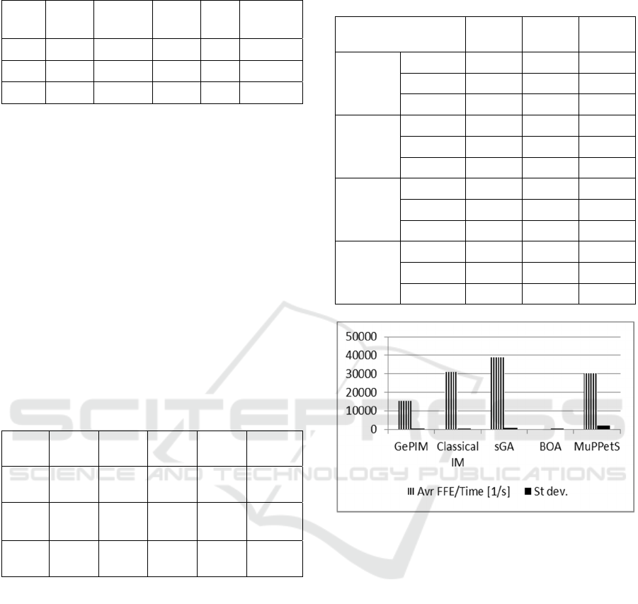
Table 9: The average time comparison.

TC no.

GePIM

[s]

Classical

IM [s]

sGA

[s]

BOA

[s]

MuPPetS

[s]

1-8 300 2624 3040 3622 4886

9-14 643 2151 1890 4410 2534

15-18 1035 3253 2941 5485 427

but GePIM and classical IM are the best. Note that

BOA reported results of very low quality for 17th

and 18th test case. To encode solutions to these test

cases 1000 genes is necessary. For such a large gene

number, the computation load spent by BOA for

building the Bayesian network (it is built at every

iteration) rises significantly and makes the method

ineffective. Similar situation, in which BOA was

unable to handle the problems encoded with large

gene number was already observed and discussed in

(Kwasnicka and Przewozniczek, 2011).

The worst solution quality for each test case type

group is reported in Table 10. The comparison

confirms that GePIM and MuPPetS are the only two

methods that guarantee the highest solution quality

for all problem types.

Table 10: The comparison of the worst solution quality for

each test case type.

GePIM

[%]

Classical

IM [%]

sGA

[%]

BOA

[%]

MuPPetS

[%]

Dec.

func.

95.00 51.67 49.83 90.00

96.00

Knap

sack

100.00 100.00

99.95 98.89 99.93

MAX-

2SAT

100.00

99.98 99.77 85.96 99.77

To confirm the statistical significance of solution

quality differences the Wilcoxon statistical test was

used. The p-values reported by this test are presented

in Table 11. The tests were performed on the results

of all runs, rounded if necessary, to the sixth most

significant position. The results obtained confirm the

analysis presented above – GePIM significantly

outperforms all competing methods except MuPPetS

for the deceptive functions concatenations case.

In Figure 2 the dependency between the computation

time and FFE for all competing methods is

presented. The comparison is done for deceptive

functions concatenations test cases (80 runs per

method). Similar comparisons may be found in (Cai

and Wang, 2015; Kwasnicka and Przewozniczek,

2011; Przewozniczek et al., 2015; Saha et al., 2010,

Suganthan et al., 2005).

Table 11: The solution quality comparisons on the base of

p-values reported by Wilcoxon test.

Null hypothesis:

GePIM...

better or

equal

worse or

equal

Classical

0 0

KS 0.50 0.50

M2S

0.85

0.16 0.33

sGA

0 0

M2S

0 0

BOA

DF 0.59 0.41

0.83

0.99

0 0

M2S

0 0

MuPPetS

DF 0.24

0.76

0.49

0 0

M2S

0 0

Figure 2: Average FFE per second for deceptive functions

concatenations.

As shown in Figure 2 the dependency between

FFE and computation time is highly repeatable – the

standard deviation value is low. The sGA is capable

of doing the highest FFE number per second. This is

an expected result since sGA does not do many

computation load consuming operations other than

fitness calculation. The high number of FFE per

second is also understandable for MuPPetS and

Classical IM. GePIM does about 50% of FFE done

by Classical IM. This difference is a result of

frequent migrations, which require many sorting

operations. Finally, the average number of FFE per

second for BOA is about 30 times lower than in the

GePIM case, which confirms the previous reasoning

that the FFE number is not a suitable computation

load measure for BOA.

ECTA 2016 - 8th International Conference on Evolutionary Computation Theory and Applications

5 CONCLUSIONS AND FURTHER

WORK

In this paper, the proposition of the Linked Gene

Groups Migration for Island Models was presented.

The GePIM method, an IM using the proposed

LGGM was shown to be an effective tool when

compared to other evolutionary methods. Despite its

simplicity, GePIM was able to compete successfully

with MuPPetS and BOA methods.

The main fields that should be concerned in the

future work are as follows:

 the application of GePIM to other problems

than those considered in this paper,

 further LGGM development,

 employing in GePIM other LL techniques

than used in this paper,

 combining the LGGM, the LL and dynamic

subpopulation number control

(Przewozniczek, 2016).

The further research in the above directions

should allow proposing new and more effective

evolutionary methods.

REFERENCES

Alves, H. N. 2015. A Multi-population Hybrid Algorithm

to Solve Multi-objective Remote Switches Placement

Problem in Distribution Networks. In Journal of

Control, Automation and Electrical Systems, 25, 5,

545-555.

Cai, Y., Wang, J. 2015. Differential evolution with hybrid

linkage crossover. In Information Sciences, 320, 244-

287.

Chang, W.D. 2015. A modified particle swarm

optimization with multiple subpopulations for

multimodal function optimization problems. In

Applied Soft Computing, 33, 170-182.

Chen, Y., Peng. W, Jian M. 2007a. Particle Swarm

Optimization With Recombination and Dynamic

Linkage Discovery. In IEEE Transactions on Systems,

Man and Cybernetics, Part B: Cybernetics, 37, 6,

1460-1470.

Chen, Y., Sastry, K., Goldberg, D.E. 2007b. A Survey of

Linkage Learning Techniques in Genetic and

Evolutionary Algorithms. In IlliGAL Report No.

2007014, Illinois Genetic Algorithms Laboratory.

Dahzi, W., Wu, C.H., Ip, W.H., Wang, D., Yan, Y. 2008.

Parallel multi-population Particle Swarm Optimization

Algorithm for the Uncapacitated Facility Location

problem using OpenMP. In IEEE Congress on

Evolutionary Computation, 124-128.

delaOssa, L., Gámez, J.A., Puerta, J.M. 2004. Migration of

Probability Models Instead of Individuals: An

Alternative When Applying the Island Model to

EDAs. In Lecture Notes in Computer Science (PPSN

2004), 3242, 242-252.

Fidrysiak, B., Przewozniczek, M. 2015. Towards Finding

an Effective Way of Discrete Problems Solving: the

Particle Swarm Optimization, Genetic Algorithm and

Linkage Learning Techniques Hybrydization. In

Proceedings of the 7th International Joint Conference

on Computational Intelligence, 228-236,

DOI=10.5220/000559660228023.

Fieldsend, J. E. 2014. Running Up Those Hills: Multi-

Modal Search with the Niching Migratory Multi-

Swarm Optimiser. In IEEE Congress on Evolutionary

Computation, 2593-2600.

Goldberg, D.E., Deb, K., Kargupta, H., Harik, G. 1993.

Rapid, Accurate Optimization of Difficult Problems

Using Fast Messy Genetic Algorithms. In Prcs. 5th

International Conference on Genetic Algorithms, 55-

64.

Kim, H.H., Choi, J.Y. 2015. Pattern generation for multi-

class LAD using iterative genetic algorithm with

flexible chromosomes and multiple populations. In

Expert Systems with Applications, 42, 833–843.

Kurdi, M. 2016. An effective new island model genetic

algorithm for job shop scheduling problem. In

Computers and Operations Research, 67, 132-142.

Kwasnicka, H., Przewozniczek, M. 2011. Multi

Population Pattern Searching Algorithm: a new

evolutionary method based on the idea of messy

Genetic Algorithm. In IEEE Transactions on

evolutionary computation, 15, 5, 715-734.

Leitão, A., Pereira, F.B., Machado, P. 2015. Island models

for cluster geometry optimization: how design options

impact effectiveness and diversity. In Journal of

Global Optimization, 63, 677-707.

Muelas, S., Mendiburu, A., LaTorre, A., Peña, J.-M. 2014.

Distributed Estimation of Distribution Algorithms for

continuous optimization: How does the exchanged

information influence their behavior? In Information

Sciences, 268, 231-254.

Omidivar, M.N., Li, X., Mei, Y., Yao, X. 2014.

Cooperative Co-evolution with Differential Grouping

for Large Scale Optimization. In IEEE Transactions

on evolutionary computation, 18, 378-393.

Pisinger, D. 2005. Where are the hard knapsack problems?

In Compuers and Operation Research. 32, 9, 2271-

2284.

DOI=http://dx.doi.org/10.1016/j.cor.2004.03.002.

Pelikan, M., Goldberg, D.E., Cantu-Paz, E. 1999. BOA:

The Bayesian Optimization Algorithm. In IlliGAL

Report No. 99003.

Pelikan, M., Sastry, K., Butz, M.V., Goldberg, D.E. 2006.

Hierarchical BOA on Random Decomposable

Problems. In MEDAL Report No. 2006001.

Przewozniczek, M., Goscien, R., Walkowiak, K.,

Klinkowski, M. 2015. Towards Solving Practical

Problems of Large Solution Space Using a Novel

Pattern Searching Hybrid Evolutionary Algorithm -

An Elastic Optical Network Optimization Case Study.

In Expert Systems with Applications, 42, 7781-7796.

Linked Genes Migration in Island Models

Przewozniczek, M. 2015. Towards finding an effective

uniform and single point crossover balance for

optimization of Elastic Optical Networks. In The

Proceedings Of The Second European Network

Intelligence Conference.

Przewozniczek, M., 2016. Active Multi Population

Pattern Searching Algorithm for Flow Optimization in

Computer Networks – the novel coevolution schema

combined with linkage learning. In Information

Sciences, 355-356, 15-36.

Saha, A., Datta, R., Deb, K. 2010. Hybrid gradient

projection based Genetic Algorithms for constrained

optimization. In IEEE Congress on Evolutionary

Computation, 1-8.

Skolicki, Z., De Jong, K. 2007. The importance of a two-

level perspective for island model design. In

Proceedings of the IEEE Congress on Evolutionary

Computation, 4623–4630.

Skolicki, Z. 2008. Linkage in Island Models. In Lecture

Notes in Computer Science, 157, 41-60.

Suganthan, P., Hansen, N., Liang, J., Deb, K., Chen, Y.,

Auger, A., Tiwari, S. 2005. Problem definitions and

evaluation criteria for the CEC 2005 special session on

real-parameter optimization. In Technical Report, 1-

50, Nanyang Technol Universiy, Singapore.

Walkowiak, K., Przewozniczek, M., Pająk, K. 2013.

Heuristic Algorithms for Survivable P2P Multicasting.

In Applied Artificial Intelligence, 27, 4, 278-303.

Wang, J., Zhang, W., Zhang, J. 2015. Cooperative

Differential Evolution With Multiple Populations for

Multiobjective Optimization. In IEEE Transactions on

Cybernetics, DOI: 10.1109/TCYB.2015.2490669 (in

press).

Watanabe, O., Yamamoto, M. 2010. Average-case

analysis for the MAX-2SAT problem. In Theoretical

Computer Science, 411, 1685-1697.

DOI=http://dx.doi.org/10.1016/j.tcs.2009.12.020.

Watson, R.A., Pollack, J.B. 1999. Hierarchically

Consistent Test Problems for Genetic Algorithms. In

Proceedings of 1999 Congress on Evolutionary

Computation, CEC-99, 2.

Watson, R.A. 2006. Compositional Evolution: The impact

of Sex, Symbiosis and Modularity on the Gradualist

Framework of Evolution. In Vienna Series in

Theoretical Biology. MIT Press.

Yang, Z., Tang, K., Yao, X. 2008. Large scale

evolutionary optimization using cooperative

coevolution. In Information Sciences, 178, 2986–2999.

Yu, T., Goldberg, D.E., Sastry, K., Lima, C.F., Pelikan,

M. 2009. Dependency structure matrix, genetic

algorithms, and effective recombination. In

Evolutionary Computation, 17, 595-626.

Zavoianu, A.-C., Lughofer, E., Bramerdorfer, G.,

Amrhein, W., Klemen, E. P. 2015. DECMO2: a robust

hybrid and adaptive multi-objective evolutionary

algorithm. In Soft Computing, 19, 12, 3551-3569.

Zhang, J., Huang, D.-S., Liu, K.-H. 2007. Multi-Sub-

Swarm Optimization Algorithm for Multimodal

Function Optimization. In IEEE Congress on

Evolutionary Computation, 3215-3220.

ECTA 2016 - 8th International Conference on Evolutionary Computation Theory and Applications