
Heterogeneous Ensemble for Imaginary Scene Classification
Saleh Alyahyan, Majed Farrash and Wenjia Wang
Computing Science, University of East Anglia, Norwich Research Park, Norwich, U.K.
Keywords:
Heterogeneous Ensemble, Diversity, Big Data, Scene Classification.
Abstract:
In data mining, identifying the best individual technique to achieve very reliable and accurate classification
has always been considered as an important but non-trivial task. This paper presents a novel approach -
heterogeneous ensemble technique, to avoid the task and also to increase the accuracy of classification. It
combines the models that are generated by using methodologically different learning algorithms and selected
with different rules of utilizing both accuracy of individual modules and also diversity among the models. The
key strategy is to select the most accurate model among all the generated models as the core model, and then
select a number of models that are more diverse from the most accurate model to build the heterogeneous
ensemble. The framework of the proposed approach has been implemented and tested on a real-world data
to classify imaginary scenes. The results show our approach outperforms other the state of the art methods,
including Bayesian network, SVM and AdaBoost.
1 INTRODUCTION
Data has been increasing rapidly not only in sheer
quantity but also in complexity and variety of multi-
media. This increase poses a significant challenge for
data mining field to develop new methods and tech-
niques to analyse and mine large datasets more ef-
fectively, including image and text data. Classifying
imaginary scenes has become a problem that many re-
searchers have been working to solve (Lazebnik et al.,
2006; Wallraven et al., 2003). Finding a solution is
crucial because such classification is used to support
myriad tasks such as localization, mapping, and nav-
igation (Siagian and Itti, 2007). Understanding scene
classification further helps to understand images and
recognize various objects in the images (Hotta, 2008).
Studies on imaginary scene classification requires two
phases. The first is to extract the features contained
in image datasets (Yang et al., 2007; Lazebnik et al.,
2006; Grauman and Darrell, 2005). The second is
to apply suitable and useful classification methods
(Yang et al., 2007; Wallraven et al., 2003), such as
ensemble.
An ensemble (Dietterich, 2000) combines multi-
ple models with the aim of achieving better results
usually via a grating technique in the field of ma-
chine learning, which can be useful for scene classi-
fication. However, when attempting to build an ef-
fective ensemble several factors need to be consid-
ered. The first factor is the accuracy gained for each
individual model in the ensemble members (Caruana
et al., 2004). The second factor is the diversity among
the member models in the ensemble (Caruana et al.,
2004) (Wang, 2008; Zenobi and Cunningham, 2001).
The third factor is the number of models that are com-
bined to build the ensemble (Zhang et al., 2005). The
decision fusion function used in the ensemble also af-
fects the results (Liu et al., 2000).
This paper presents a heterogeneous ensemble for
scene classification because it is a complex multiple-
class problem that has overwhelmed single models
but could be better dealt with ensemble methods to
achieve two benefits. One benefit is that an ensem-
ble is more likely to outperform individual models
(Brown et al., 2005; Wang et al., 2003). Another ben-
efit of an ensemble is the reliability it offers (Wang,
2008). Using this problem as a case study, this work
also investigates how much the ensemble members
affect the accuracy of the results of imaginary scene
classification, in terms of the accuracy of the individ-
ual models selected, the diversity among the models,
and the size of the ensemble.
The rest of the paper is organized as follows. Sec-
tion 2 will briefly discuss several of the previous stud-
ies in the field. Section 3 will detail our methods, list-
ing the tools and programs used in the research. Sec-
tion 4 provides details of the experiment conducted
and our results. Section 5 will present our conclusions
and suggestions for the future work.
Alyahyan, S., Farrash, M. and Wang, W.
Heterogeneous Ensemble for Imaginary Scene Classification.
DOI: 10.5220/0006037101970204
In Proceedings of the 8th International Joint Conference on Knowledge Discovery, Knowledge Engineering and Knowledge Management (IC3K 2016) - Volume 1: KDIR, pages 197-204
ISBN: 978-989-758-203-5
Copyright
c
2016 by SCITEPRESS – Science and Technology Publications, Lda. All rights reserved
197
2 RELATED WORK
Many scene classification studies have been previ-
ously conducted. A notable study was done by (Oliva
and Torralba, 2001) using a dataset called 8 Scene
Categories Dataset. Their experiment involved clas-
sifying images and their annotations into eight cate-
gories using the support vector machine technique, by
training 100 instances from each class and testing the
rest. They achieved 83.70% accuracy.
(Bosch et al., 2006) also studied scene classifica-
tion. They started the study by recognizing all pos-
sible objects in the image, and then classifying each
image regrading to its objects. They used pLSA (Hof-
mann, 2001) to represent objects in the images. The
pLSA originally devolved as topic discovery in a text
but it was used in this research because images were
represented as frequency of visual words. The k-
Nearest Neighbour (k-NN) algorithm was used as a
classification method in three different datasets.
(Yang et al., 2007) conducted an experiment on
scene classification using keypoint as a method to ex-
tract features from images. In their experiment, im-
ages were described as a bag of visual words. They
demonstrated that their methods outperform others
using two benchmark datasets: TRECVID 2005 cor-
pus and PASCAL 2005 corpus. The keypoint ap-
proach was originally created to classify text datasets,
and was found to be useful for image classification as
conducted in this experiment and others, including in
(Lowe, 2004), (Ke and Sukthankar, 2004), (Mikola-
jczyk and Schmid, 2004).
(Lertampaiporn et al., 2013) applied a heteroge-
neous ensemble for pre-miRNA in their experiment
by using voting for a set of classifiers including a sup-
port vector machine, k-NN and random forests.
Scene classification has been studied from the
view of homogeneous ensemble methods. (Yan et al.,
2003) applied an homogeneous ensemble of SVM
models to classify rare classes on scene classification.
Their experiment was conducted on a dataset called
(TREC 02 Video Track), and was compared with
other approaches applied to the same dataset. The re-
sults obtained in the experiment outperformed other
methods with 11% improvement in the best case.
(Giacinto and Roli, 2001)enforced neural network
ensemble for image classification on a dataset of
multi-sensor remote-sensing images. They focused
on classifying a bunch of pixels related to different
images for different classes. The experimental results
they obtained demonstrated the effectiveness of ho-
mogeneous neural network ensemble, with the level
of accuracy achieved in the experiment being higher
than the best accuracy of individual neural network
models.
In summary, the previous studies used different
features and methods for scene classification , but
these studies were limited in terms of the type of fea-
tures extracted from images and the methods used as
most experiments were conducted using just one clas-
sification model, for example support vector machine
and k-NN approaches, whilst other studies used ho-
mogeneous ensemble. Heterogeneous ensemble was
not used for classifying image scene.
3 THE HETEROGENEOUS
ENSEMBLE SYSTEM (HES)
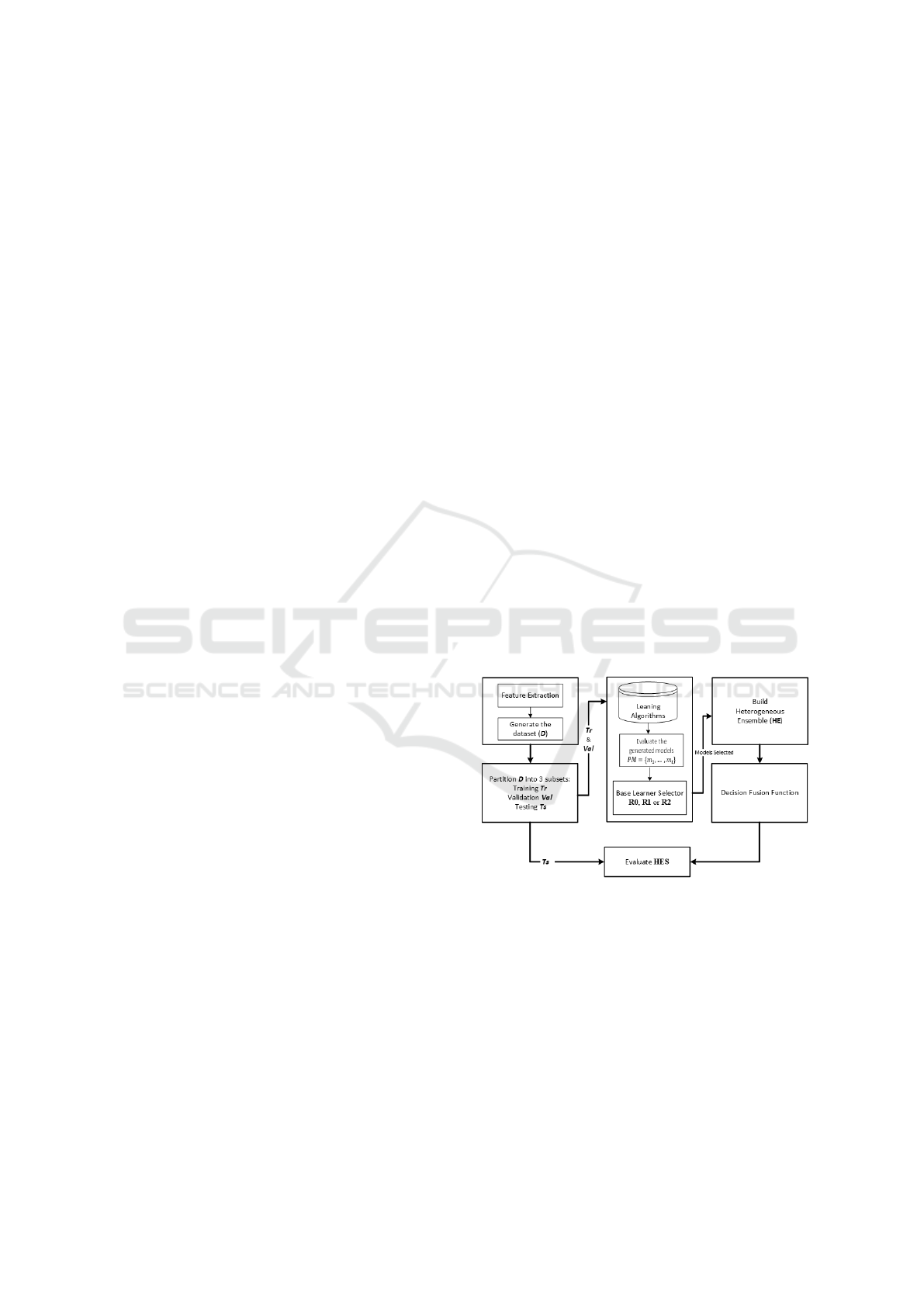
3.1 The Framework of the HES
The proposed heterogeneous ensemble system as
shown in Fig.1, consists five main components: 1,
feature extraction and data formation; 2, data parti-
tion; 3, heterogeneous model generation and evalua-
tion; 4, ensemble construction and 5, decision fusion
function. The key idea of the proposed heterogeneous
ensemble system (HES) is to generate methodolog-
ically different models, hence called heterogeneous
models, by different learning algorithms, as the mem-
ber candidates and then build an ensemble with the
rules as defined below.
Figure 1: The general framework for HES.
The main operations of the HES are shown by
Algorithm (1). It starts by dividing D into training
dataset and testing dataset Ts. The training dataset
was further divided to train dataset Tr for training
the classifiers C
i
∈ C and validation dataset Val for
evaluating each C
i
. Different learning algorithms are
called from the learning algorithms base to generate
|
C
|
models,which are stored in a model pool PM.
KDIR 2016 - 8th International Conference on Knowledge Discovery and Information Retrieval
198

Algorithm 1: Algorithm for Building HES.
1: Input: D dataset, C base learners, ensemble size
|
Φ
|
and the selected rule R.
2: Output: Acc(HES).
3: Divide D to Train 75% and Ts 25%
4: Divide the training data to Tr 75% and Val 25%
5: let N =
|
Φ
|
6: for i = 1 to
|
C
|
do
7: m
i
= model resulted from training Tr on C
i
8: add m
i
to PM
9: Evaluate m
i
on Val
10: end for
11: Call the selected rule R
12: Evaluate HES on Ts
3.2 Rules for Building Different HES
Different rules can be devised to build various hetero-
geneous ensembles based on different strategies and
purposes. Three rules R0, R1, and R2 are defined in
this study as the demonstration of concept in utilising
the accuracy as a model selection criterion alone, or
both accuracy and diversity measures.
Fig.2. shows all the three rules and the details of
these rules are described as follows.
Figure 2: Main steps for R0, R1 and R2 in HES.
3.2.1 Rule R0:
To build an HES, this rule only considers the accuracy
of individual models only. Algorithm (2) describes
how it works where the HES will first sort models in
the PM in a descending order according to the accu-
racy of each individual model Acc(m
i
) on Val. Then,
the most accurate N models are selected from PM to
be added to Φ. This is the basic rule applied in HES,
and also forms a part of all other rules in the system.
Fig. 2a illustrates how this rule works. To select the
models we need to use equation (1).
m
i
= max
Acc(m
j
), m
j
∈ PM
i = 1...N (1)
Algorithm 2: Algorithm for R0.
1: Input: PM
2: Output: The selected models
3: sort models in the PM decreasingly according to
acc(m
i
)
4: select first N models from PM
5: add selected models to Φ
3.2.2 Rule R1:
To build an HES, this rule considers both accuracy
and diversity measured by pair-wise diversity. Algo-
rithm (3) describes how it works. In this rule, HES
first selects the most accurate model MAM from PM
to be added to Φ. Then this model is removed from
the pool PM.
m
1
= max
Acc(m
j
), m
j
∈ PM
(2)
Then, the diversity measured by (Double-
Fault)DF (Giacinto and Roli, 2001) between MAM
and every model in the pool PM is calculated using
a pairwise strategy to fill the models needed for the
finalΦ. Then PM is sorted in the decreasing order
according to their diversity DF to select N-1 most di-
verse models from the pool PM to be added to the
final Φ. Equation(3) is applied for this stage. The
models selected in this rule are MAM and N-1 most
diverse models from MAM in the pool PM. Fig.2b,
illustrates how this rule works.
m
i
= max
DF(m
1
, m
j
), m
j
∈ PM
i = 2...N (3)
Algorithm 3: Algorithm for R1.
1: Input: PM
2: Output: The selected models
3: MAM=the most accurate model in PM
4: add MAM to Φ
5: remove MAM from PM
6: for i = 1 to
|
PM
|
do
7: calculate DF diversity (MAM ,m
i
)
8: end for
9: sort PM decreasingly according to their diversity
10: select first (N-1)models
11: add selected models to Φ
3.2.3 Rule R2:
This rule uses both accuracy and two diversity mea-
sures: DF and (Coincident Failure Diversity) CFD
(Partridge and Krzanowski, 1997). Algorithm (4) de-
scribes the procedure of R2. In this rule, the first
model m
1
to be selected for the Φ is chosen as in equa-
tion (2) in R1, which is MAM. The second model m
2
to be selected for Φ is the most diverse model MDM
Heterogeneous Ensemble for Imaginary Scene Classification
199

from the most accurate model in the pool PM. To cal-
culate MDM, equation (4) is used.
m
2
= max
DF(m
1
, m
j
), m
j
∈ PM
(4)
In this rule, we generate a number of combina-
torics J, subsets of models φ
i
from the pool of models
PM and equation (5) to calculate this number.
J =
|
PM
|
N − 2
(5)
Each combinatory φ
i
includes MAM and MDM,
and the remaining models needed to reach to N are
added from the pool PM to compute the diversity
CFD. Thus the maximum diverse subset φ
i
ensemble
is chosen for the final Φ. Fig.2c, illustrates how this
rule works.
HES = max
CFD(Φ ⇐ m
j
), m
j
∈ PM
(6)
Algorithm 4: Algorithm for R2.
1: Input: PM
2: Output: The selected models
3: MAM=the most accurate model in PM
4: remove MAM from PM
5: for i = 1 to
|
PM
|
do
6: calculate DF diversity (MAM ,m
i
)
7: end for
8: MDM = the most divers model from MAM
9: remove MDM from PM
10: J= The number of Combinations subsets
|
PM
|
N−2
11: for i = 1 toj do
12: φ
i
=the i
th
combinations subset from PM
13: add MAM and MDM to φ
i
14: calculate CFD diversity φ
i
15: end for
16: add the most divers φ
i
to Φ
3.3 Implemetation of HES
The HES is implemented with Java, based on Weka
API. Thus, the experiment was carried out on a nor-
mal PC, with an I7 processor and 16 GB RAM.
As HES is flexible for selecting candidate classi-
fiers, we have selected 11 deferent base classifiers
that are provided in the WEKA library. These
base classifiers are: trees(J48, RandomTree, REP-
Tree), bayes(NaiveBayes, BayesNet), function(SMO),
rules(JRip, PART) and Lazy(IBk, LWL, KStar).
4 EXPERIMENT DESIGN AND
RESULTS
4.1 Dataset
We conducted our experiment using a benchmark
dataset called 8 Scene Categories Dataset (Oliva and
Torralba, 2001),which was divided into two parts: im-
ages and their annotations. The relevant part is in
the annotation folder which, contains 2688 XML files
categorized into eight groups, and each XML file con-
tains a number of tags that describe an image.The an-
notations were dealt with as text and used in this in-
expedient. The features were extracted from this text,
and we obtained 2866 instances, 782 attributes and 8
classes.
4.2 Experiment Design and Results
We conducted a series of experiments investigating
three rules in HES. They are generated by changing
two factors. The first is the rule used in the experi-
ment, which are R0, R1 and R2. The second is the
ensemble size, which are 3, 5, 7 and 9. Running all
possible combination of these parameters, and repeat-
ing them for five different runs lead to conduct 60 ex-
periments in total.
The results (mean and standard deviation) of using
R0, R1 and R2 with different numbers of models in
HES are shown in Fig.3,4 and 5, over 5 runs on each
figure.
The results for all five runs on all three rules are
about as accurate as those of the most accurate model
MAM but more reliable because the single best model
varied in different runs and could be much worse in
some runs. In this study the most accurate model was
not stable for all the five runs it some times BayesNet
and other times SMO. This negatively impacts relia-
bility. Thus, ensemble accuracy wins against the most
accurate model in certain instances.
The most significant finding from applying the
three rules was the stable improvement of the level
of the accuracy when R2 is applied, as seen in Fig.
5. The observable reason for that is R2 considers
more diversity measures than R0 and R1. Consider-
ing more diverse models provided an opportunity to
achieve stable results even if the mean accuracy for
these models was low. This is a clear evidence that
can increase reliability whilst maintaining high accu-
racy.
Another observable finding from the results is that
increasing the number of models used in the ensemble
supported with the diversity among them lead to more
stable results, as shown in Fig. 5. For R2, when more
than five models were selected for the ensemble, the
results became more stable.
When there were three models in R2, the accuracy
was lower than for the other rules. That was probably
because when the size of an HES is as small as 3,
adding a more diverse but less accurate model to it,
the diversity introduced is not enough to compensate
KDIR 2016 - 8th International Conference on Knowledge Discovery and Information Retrieval
200
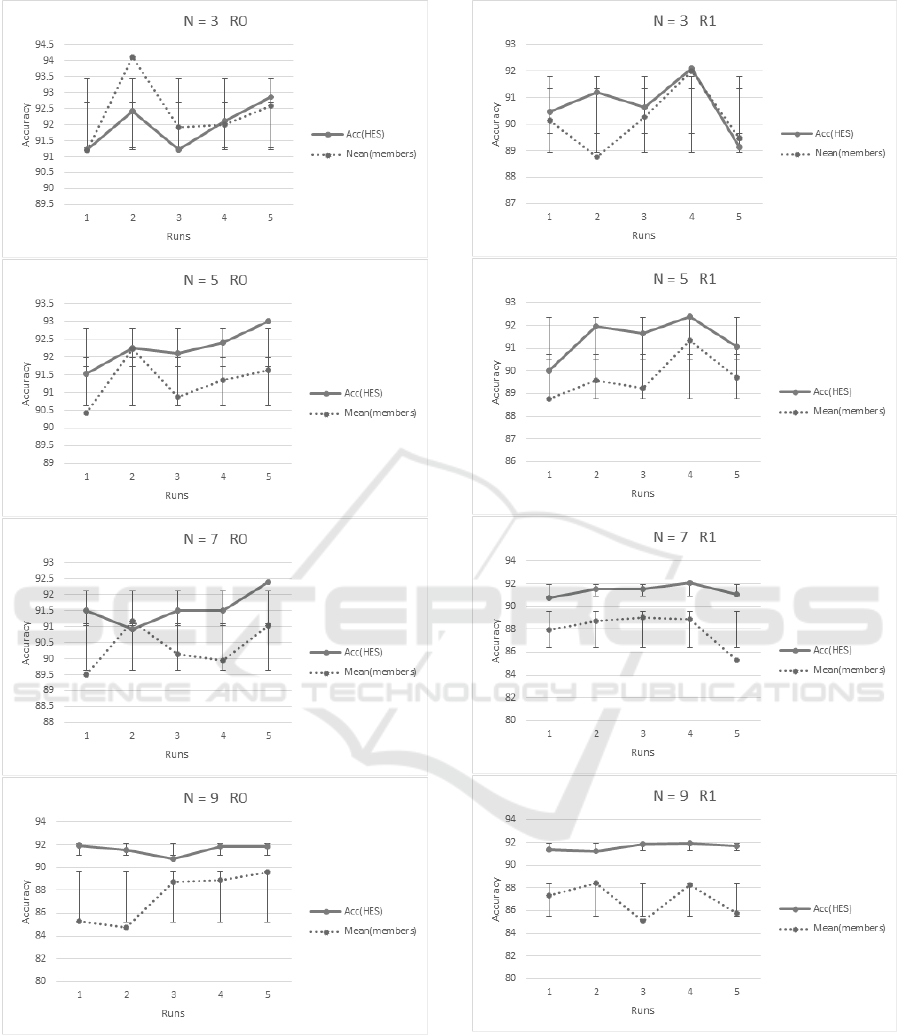
Figure 3: All HES results for the rule R0. The size of
ensemble 3, 5, 7 and 9 are shown in each sub-graph re-
spectively. Tow lines (solid and dashed) are the accuracy
of HES and the mean accuracy for models that are chosen
for the HES respectively. The stranded deviation is shown
whiskers over 5 runs.
the loss of the accuracy caused by the third less accu-
rate mode, so the chance for using the diversity mea-
Figure 4: All HES results for the rule R1. The size of
ensemble 3, 5, 7 and 9 are shown in each sub-graph re-
spectively. Tow lines (solid and dashed) are the accuracy
of HES and the mean accuracy for models that are chosen
for the HES respectively. The stranded deviation is shown
whiskers over 5 runs.
sure is more likely to be effective when the number
of models for the ensemble is increasing.
Heterogeneous Ensemble for Imaginary Scene Classification
201

Figure 5: All HES results for the rule R2. The size of
ensemble 3, 5, 7 and 9 are shown in each sub-graph re-
spectively. Tow lines (solid and dashed) are the accuracy
of HES and the mean accuracy for models that are chosen
for the HES respectively. The stranded deviation is shown
whiskers over 5 runs.
Figure 6: Comparing all three rules in four different sizes
of the HES.
4.3 Comparison of the Results
The comparison was carried out with some other en-
semble methods, including various homogeneous en-
semble built with AdaBoost algorithm for each base
classifier used in HES.
Table 1 shows the mean results for homogeneous
ensemble over all the five runs conducted. It can
be seen that these homogeneous ensembles produced
quite different or unstable accuracy for the task with
the highest up to 90.83% and lowest down to 77.74%.
Table 1: The mean of the accuracy for five runs using Ad-
aBoostM1 method for each base classifier in HES.
Base Classifier Mean Accuracy SD
J48 89.61 0.80
RandomTree 84.26 184
REP-Tree 88.33 0.52
NaiveBayes 90.71 0.44
BayesNet 90.57 0.65
SMO 90.83 0.27
JRip 88.24 0.32
PART 89.23 0.60
IBk 86.37 0.62
LWL 77.74 4.01
KStar 86.76 0.69
Table 2 shows the comparison between the homo-
geneous ensemble and (R0, R1 and R3) in HES. It is
very clear that heterogeneous ensemble constructed
by any of the three rules are the best and improved
the average accuracy as much as 3.5%.
Table 2: The comparison results between the homogeneous
ensemble and HES for all the three rules.
Mean Accuracy SD
homogeneous Ensemble 87.51 3.84
Rule R0 91.85 0.33
Rule R1 91.29 0.39
Rule R2 91.29 1.37
KDIR 2016 - 8th International Conference on Knowledge Discovery and Information Retrieval
202

5 CONCLUSION AND FUTURE
WORK
This study used an imaginary scene classification
problem as a testing case to investigate the capability
of heterogeneous ensembles built with the ruls that
consider either accuracy of individual models or di-
versity, or both.Three rules are devised specifically
using accuracy of individual models and the diver-
sity measurements among these models for an en-
semble.The results for HES are much better than the
previous studies (Oliva and Torralba, 2001) that used
individual models for imaginary scene classification
and the state-of-the-art for the homogeneous ensem-
ble, which used all base classifiers used in HES. The
increasing diversity among the models selected for
the ensemble was found to be advantageous, lead-
ing to more stable and reliable results. Our research
found that increasing the number of models also af-
fects the ensembles results. This indicated that diver-
sity is more effective when used with a higher number
of models selected for the ensemble. It can therefore
be concluded that combining models results in high
accuracy and diversity for an ensemble has consider-
able advantages in terms of the ensemble’s accuracy.
Various questions for future work emerge from
this paper. First, this research covered only the anno-
tations part of the dataset. It could be useful to involve
the images part directly. Second, only three rules were
used in this experiment; future work should consider
more rules with different measures for ensemble se-
lecting models. Third, more experiments will be con-
ducted by using more datasets.
REFERENCES
Bosch, A., Zisserman, A., and Mu
˜
noz, X. (2006). Scene
classification via plsa. In Computer Vision–ECCV
2006, pages 517–530. Springer.
Brown, G., Wyatt, J., Harris, R., and Yao, X. (2005). Di-
versity creation methods: a survey and categorisation.
Information Fusion, 6(1):5–20.
Caruana, R., Niculescu-Mizil, A., Crew, G., and Ksikes, A.
(2004). Ensemble selection from libraries of models.
In Proceedings of the twenty-first international con-
ference on Machine learning, page 18. ACM.
Dietterich, T. G. (2000). Ensemble methods in machine
learning, pages 1–15. Springer.
Giacinto, G. and Roli, F. (2001). Design of effective neural
network ensembles for image classification purposes.
Image and Vision Computing, 19(9):699–707.
Grauman, K. and Darrell, T. (2005). The pyramid match
kernel: Discriminative classification with sets of im-
age features. In Computer Vision, 2005. ICCV 2005.
Tenth IEEE International Conference on, volume 2,
pages 1458–1465. IEEE.
Hofmann, T. (2001). Unsupervised learning by probabilis-
tic latent semantic analysis. Machine learning, 42(1-
2):177–196.
Hotta, K. (2008). Scene classification based on multi-
resolution orientation histogram of gabor features. In
Computer Vision Systems, pages 291–301. Springer.
Ke, Y. and Sukthankar, R. (2004). Pca-sift: A more
distinctive representation for local image descriptors.
In Computer Vision and Pattern Recognition, 2004.
CVPR 2004. Proceedings of the 2004 IEEE Computer
Society Conference on, volume 2, pages II–506. IEEE.
Lazebnik, S., Schmid, C., and Ponce, J. (2006). Beyond
bags of features: Spatial pyramid matching for rec-
ognizing natural scene categories. In Computer Vi-
sion and Pattern Recognition, 2006 IEEE Computer
Society Conference on, volume 2, pages 2169–2178.
IEEE.
Lertampaiporn, S., Thammarongtham, C., Nukoolkit, C.,
Kaewkamnerdpong, B., and Ruengjitchatchawalya,
M. (2013). Heterogeneous ensemble approach with
discriminative features and modified-smotebagging
for pre-mirna classification. Nucleic acids research,
41(1):e21–e21.
Liu, Y., Yao, X., and Higuchi, T. (2000). Evolutionary en-
sembles with negative correlation learning. Evolution-
ary Computation, IEEE Transactions on, 4(4):380–
387.
Lowe, D. G. (2004). Distinctive image features from scale-
invariant keypoints. International journal of computer
vision, 60(2):91–110.
Mikolajczyk, K. and Schmid, C. (2004). Scale & affine in-
variant interest point detectors. International journal
of computer vision, 60(1):63–86.
Oliva, A. and Torralba, A. (2001). Modeling the shape
of the scene: A holistic representation of the spatial
envelope. International journal of computer vision,
42(3):145–175.
Partridge, D. and Krzanowski, W. (1997). Software di-
versity: practical statistics for its measurement and
exploitation. Information and software technology,
39(10):707–717.
Siagian, C. and Itti, L. (2007). Rapid biologically-inspired
scene classification using features shared with visual
attention. Pattern Analysis and Machine Intelligence,
IEEE Transactions on, 29(2):300–312.
Wallraven, C., Caputo, B., and Graf, A. (2003). Recognition
with local features: the kernel recipe. In Computer
Vision, 2003. Proceedings. Ninth IEEE International
Conference on, pages 257–264. IEEE.
Wang, H., Fan, W., Yu, P. S., and Han, J. (2003). Mining
concept-drifting data streams using ensemble classi-
fiers. In Proceedings of the ninth ACM SIGKDD in-
ternational conference on Knowledge discovery and
data mining, pages 226–235. ACM.
Wang, W. (2008). Some fundamental issues in ensem-
ble methods. In Neural Networks, 2008. IJCNN
2008.(IEEE World Congress on Computational In-
Heterogeneous Ensemble for Imaginary Scene Classification
203

telligence). IEEE International Joint Conference on,
pages 2243–2250. IEEE.
Yan, R., Liu, Y., Jin, R., and Hauptmann, A. (2003). On
predicting rare classes with svm ensembles in scene
classification. In Acoustics, Speech, and Signal Pro-
cessing, 2003. Proceedings.(ICASSP’03). 2003 IEEE
International Conference on, volume 3, pages III–21.
IEEE.
Yang, J., Jiang, Y.-G., Hauptmann, A. G., and Ngo, C.-W.
(2007). Evaluating bag-of-visual-words representa-
tions in scene classification. In Proceedings of the
international workshop on Workshop on multimedia
information retrieval, pages 197–206. ACM.
Zenobi, G. and Cunningham, P. (2001). Using diversity
in preparing ensembles of classifiers based on differ-
ent feature subsets to minimize generalization error,
pages 576–587. Springer.
Zhang, S., Cohen, I., Goldszmidt, M., Symons, J., and Fox,
A. (2005). Ensembles of models for automated diag-
nosis of system performance problems. In Depend-
able Systems and Networks, 2005. DSN 2005. Pro-
ceedings. International Conference on, pages 644–
653. IEEE.
KDIR 2016 - 8th International Conference on Knowledge Discovery and Information Retrieval
204
