
Enhanced Genetic Algorithm for Mobile Robot Path Planning in
Static and Dynamic Environment
Hanan Alsouly and Hachemi Bennaceur
Computer Science Department, Al-lmam Muhammad Ibn Saud Islamic University, Riyadh, Saudi Arabia
Keywords: Genetic Algorithm, Path Planning, Mobile Robot, Dynamic Environment, Static Environment.
Abstract: Path planning is an important component for a mobile robot to be able to do its job in different types of
environments. Furthermore, determining the safest and shortest path from the start location to a desired
destination, intelligently and in quickly, is a major challenge, especially in a dynamic environment.
Therefore, various optimisation methods are recommended to solve the problem, one of these being a
genetic algorithm (GA). This paper investigates the capabilities of GA for solving the path planning
problem for mobile robots in static and dynamic environments. First, it studies the different GA approaches.
Then, it carefully designs a new GA with intelligent crossover to optimise the search process in static and
dynamic environments. It also conducts a comprehensive statistical evaluation of the proposed GA approach
in terms of solution quality and execution time, comparing it against the well-known A* algorithm and
MGA in a static scenario, and against the Improved GA in a dynamic scenario. The simulation results show
that the proposed GA is able to find an optimal or near optimal solution with fast execution time compared
to the three other algorithms, especially in large problems.
1 INTRODUCTION
The robotics field has received a great deal of
attention from many people beside those in research
and industrial communities (Elshamli et al., 2004).
The wide variety of robotics applications is a natural
motivator for people to study this area and
contribute to it. Building sophisticated and
intelligent robots that can change the world is the
aim of everyone working in the field. The building
of intelligent robots began with basic intelligence,
models which could only move around and perform
a small set of tasks. Today, these robots outperform
humans in various kinds of tasks in terms of
efficiency and accuracy (Tiwari et al., 2012).
However, there remain several challenges to
building a complete intelligent robot. One of these
challenges is intelligently determining its fastest and
safest route to its destination. This is what is known
as the path planning problem (Elshamli et al., 2004).
The path planning problem addresses two types of
environment, static and dynamic (Miao, 2009). The
environment is called static when its information
cannot change during the robot planning and
navigation. On other hand, if the environment does
change while the robot is deliberating, then it is
called dynamic environment (Russell and Norvig,
2002). The changes may occur at the goal position,
obstacle location, or entering a new obstacle (Tiwari
et al., 2012). Path planning is an important
component for a mobile robot to be able to perform
assigned tasks in different types of environments.
The robot path planning problem is not an easy task
to solve because it has a number of issues that may
affect the efficiency of the path planning algorithm
(Tiwari et al., 2012; Chaari et al., 2012):
completeness, computational time, optimality of the
path, the path smoothness and energy consumption.
In this paper, we would like to deal with the
issue of how these robots might intelligently plan
their path in a static and dynamic environment by
using genetic algorithm. We chose to study this
problem because the current solutions suffer from
several drawbacks, among them high computation
expense, inflexibility in responding to changes in the
environment or to different optimisation goals.
Genetic algorithm was chosen because its efficiency
has been proven in many optimisation and static
path planning problems. In this paper, we study the
use of genetic algorithm in that problem.
Furthermore, we suggest a new algorithm that not
only focus on the optimality of the path but also
Alsouly, H. and Bennaceur, H.
Enhanced Genetic Algorithm for Mobile Robot Path Planning in Static and Dynamic Environment.
DOI: 10.5220/0006033401210131
In Proceedings of the 8th International Joint Conference on Computational Intelligence (IJCCI 2016) - Volume 1: ECTA, pages 121-131
ISBN: 978-989-758-201-1
Copyright
c
2016 by SCITEPRESS – Science and Technology Publications, Lda. All rights reserved
121

reduce the real-time execution for large problems, as
this is a critical criterion in mobile robots path
planning. The new algorithm is enhanced by
designing a new intelligent crossover and a set of
mutations. In addition, we test the new algorithm
and conduct a comparison study between some of
existing solutions.
The remaining parts of this paper are organised
as follows: section 2 reviews related works. Section
3 introduces our algorithm and explains its
components, while section 4 presents a comparative
study between the algorithms, evaluates
performance, reports results and discusses them.
Finally, section 5 concludes with a summary of
contributions and makes suggestions for future
research work.
2 RELATED WORK
Genetic algorithm (GA) is one of the heuristic
search algorithms. The heuristic search algorithms
do not guarantee to find a solution, but when they
do, they do it so much faster than classic search
algorithms (Masehian and Sedighizadeh, 2007). GA
proposed in 1975 by John Holland at the University
of Michigan. It is used to generate useful solutions
to optimisation, search problems and machine
learning (Hussein et al., 2012). GA belongs to the
evolutionary algorithms, which generate solutions
by using inspired techniques from natural evolution,
such as inheritance, mutation, selection, and
crossover (Reshamwala and Vinchurkar, 2013). Due
to the robustness and effectiveness of GA in several
optimisation problems, various studies have been
done to use GA in robot path planning problems.
(Elshamli et al., 2004) proposed a GA planner that
can solve the robot path planning problem in a
dynamic environment that may presents new
obstacles. To model the search space, they used
polygonal representation. The proposed algorithm
uses a variable length of chromosome and generates
random feasible initial population. For the crossover,
the algorithm uses a random one-point crossover,
whereas the mutation operation changes a node
value randomly. To solve the dynamic aspect, the
authors used four techniques, the best being Memory
and Random Immigrants. In addition, this algorithm
takes into consideration path smoothness. It has
many operations besides the basic ones, such as
Repair, Shortcut and Smooth operators.
Consequently, it takes a long time to find an optimal
or near optimal path. Therefore, (Koryakovskiy et
al., 2009) suggested eliminating the use of Repair,
Shortcut and Smooth operators, and using 3-point
interpolation by Bezier curves instead to generate
smooth paths in the initial population. The suggested
method reduces the time in finding the target path.
However, the proposed method works only in a
well-known environment with static and new
obstacles.
On other hand, (Mahjoubi et al., 2006) also used
polygonal representation for the obstacles as a
search space to make the search faster. To evaluate
the individual, the algorithm uses a fitness function
that depends on the path’s total length and penalty
factor for collision parts. This algorithm uses three
types of mutation operators: delete, insert and
change node mutation operators. This method
supports well-known environment with moving
obstacle only. (Zou et al., 2012) also suggested
improving the environment modelling by using a
grid size-adjustment technique, which can zoom-in
and zoom-out from the grid map to provide an
accurate and fast search map. Furthermore, the
authors used a nonlinear fitness function to improve
the convergence and operational efficiency of the
algorithm. In addition, (Shi and Cui, 2010) have
used a new modelling method to speed up the
execution of searching. The new method projects the
two dimensional data to one dimensional data,
which helps to reduce the size of the search space
and the size of the chromosomes. Their fitness
function depends on the path length, path security
and path smoothness. The suggested method can be
used to solve the problem in an unknown dynamic
environment.
(Zhao and Gu, 2013) devised a different idea to
solve the problem. They suggested using a two-layer
GA mechanism. In this method, each layer has
different fitness functions. The first layer is
responsible for static obstacles avoidance, while the
second layer is responsible for dynamic obstacles
avoidance. Beside of that, a new operation known as
Delete operation is used to delete the redundant bits
in the individual and the bits between them. (Yun et
al., 2011) provide an algorithm that avoids acute
obstacles in the dynamic environment. The provided
solution prevents the robot from being trapped in an
acute ‘U’ or ‘V’ shaped obstacle. In addition, this
solution handles static, dynamic and new obstacles.
When new obstacles are detected, the algorithm re-
plans the path from the current position.
Furthermore, (Zhu et al., 2015) invented a helpful
new idea for global path planning and well-known
environment. In their solution, the path is
represented as a sequence of straight-line segments,
which connect the obstacles’ vertices that are
ECTA 2016 - 8th International Conference on Evolutionary Computation Theory and Applications
122
bypassed by the path. The method limits the search
space in the space of obstacles. Furthermore, after
each crossover and mutation, the path refinement
function is applied to the child chromosomes to
correct the collide parts and enhance the quality of
the paths.
This paper in addition to proposing a new GA
and using a new environment representation method,
it is different from these works in that it evaluates
the performance of the GA on semi-large-size maps
starting from 100*100 up to 500*500.
3 DYNAMIC GENETIC
ALGORITHM
The aim of our paper is to find a practical approach
to solve a path planning problem in a dynamic
environment by using GA. To achieve that, we have
designed a new GA planner that depends on a grid-
based map to represent the environment with
polygonal representation for the obstacles. The
following subsections describes the environment
representation and the new planner.
3.1 Environment Representation
In our work, we have selected a grid-based map to
represent the environment with polygonal
representation for the obstacles. By this means, we
could cover the environment completely and update
it easily. Beside of that, polygonal representation
helps to reduce the use of the memory, to produce
smoother paths, and we can use efficient and simple
geometric algorithms (O'Rourke, 1998) (Sunday,
2012) to check the feasibility of the paths and reduce
the computational complexity.
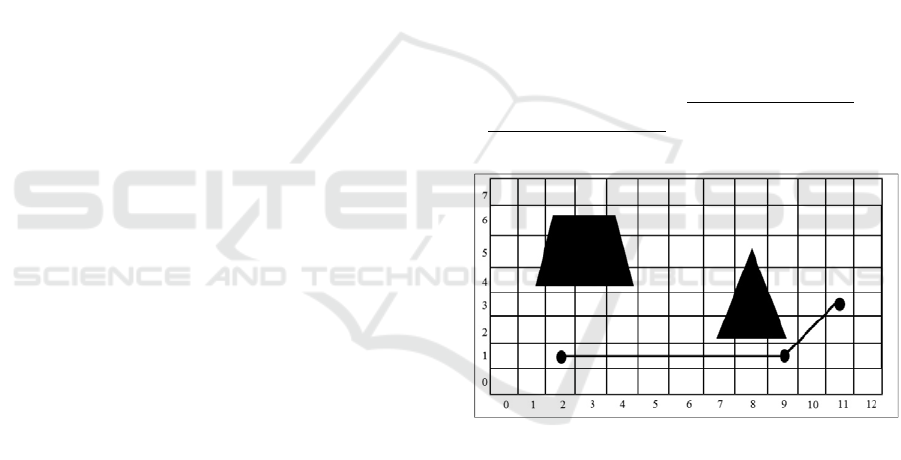
3.1.1 Grid Representation
The used grid map represents the environment in a
2D way by dividing it into equal square cells, as
shown in figure 1. Each cell has a coordinate
number. We assume the environment is rectangular
and its boundary is static. In addition, the mobile
robot can move from one cell to another free cell in
a straight line if the line between them does not
collide with any obstacle.
3.1.2 Obstacles Representation
We assume the obstacles are polygons, and they are
represented by the ordered list of its vertices. Each
vertex represents cell coordination on the grid map.
Obstacle segments are constructed by connecting
these vertices, starting with the first vertex and
ending with connecting the last vertex to the first
one. For example, the first obstacle in figure 1 is
represented as [(1,4), (4,4), (4,6), (2,6)].
3.1.3 Solution Encoding
The paths encoding is one of the most important
issues for GA, because the encoding may affect GA
performance and memory performance. Since the
paths may have variable lengths and line segments,
we have chose to use a variable size solution
encoding. The solution is represented by a
chromosome. The chromosome consists of a
sequence of ordered positions that represent the line
segments, starting from the initial point and ending
at the goal point. Euclidean distance is used to count
the path cost. This method has been used to reduce
the size of the memory and to help making smooth
paths. Figure 1 shows an example of a feasible path.
The path is encoded as [(2,1), (9,1), (11,3)], the
initial cell is (2,1), the goal cell is (11,3) and the cost
of the path is=
29
11
+
911
13
= 9.83.
Figure 1: Grid representation.
3.2 Genetic Algorithm Designing
To design efficient GA, we need to take care in
designing all of its parameters and operators,
because they affect the performance of a GA and
they are interrelated. In the following subsections,
we will describe how we designed these important
parameters and operators.
3.2.1 Initial Population
Generating an initial population is the first step in
the functioning of a GA. Each member of this
population encodes a possible solution to the
problem or may lead to finding the solution. In our
Enhanced Genetic Algorithm for Mobile Robot Path Planning in Static and Dynamic Environment
123

algorithm, part of initial population is generated
completely randomly. The number of cells in any
random given path is assigned randomly. In
addition, the cells’ coordinates are generated
randomly, but they must be feasible cells (outside
occupied space). The generated paths may contain
feasible and infeasible segments (intersect with
obstacles). The second part of the initial population
is generated by one-point crossover. We have used
these approaches in generating the initial population
to get a diverse population with paths of various
quality in fast time and ensure that some paths
intersected with others to help performing the
intelligent crossover in later stage.
3.2.2 Fitness Function
The value of the fitness function determines the path
cost of a chromosome. Therefore, all problem
objectives must be considered. In this paper, our
objective is to generate the shortest possible path in
acceptable time. Therefore, the same objective has
been used in the definition of the fitness function as
with the method used by (Mahjoubi et al., 2006).
This fitness function calculates the Euclidean
distance between successive points of each
chromosome and adds the results to each other. This
represents the length of each feasible chromosome.
However, the fitness of a chromosome with
collisions should be higher than the worst feasible
chromosome. The cost for path p with n cells is
defined by:
,
∗
(1)
where C(p) is the calculated cost for path p, D(A, B)
is the Euclidean distance between point A and point
B, L( p) is the total length of the collided parts in
path p, Pi is the i
th
point in the corresponding
sequence of path p (i=1, 2…, n), and M is the
penalty factor.
3.2.3 Selection Operators
The selection operator selects the best individuals
from the population to spawn a new generation of
the population. In this paper, we used two selection
operators. Elitist selection is used to move the best
individuals in the current generation to the next
generation without any change. The elitist selection
is used to avoid losing the best paths because of the
genetic operator’s randomness (Al-Ajlan et al.,
2013). In addition, the tournament selection is used
to select a group of individuals from the population
randomly. These individuals are ranked according to
their relative fitness, and the fittest individuals is
selected to produce the next generation. The
tournament selection is used because it gives each
individual a chance to be selected even the infeasible
paths, as a result, the diversity of the population
increases (Elshamli et al., 2004).
3.2.4 Crossover Operators
The crossover operator is primarily responsible for
improving the generations to obtain the best paths.
The improvement is achieved by recombining two or
more individuals called parents to generate better
solutions called offspring. In this paper, we proposed
a new crossover operator called intelligent
crossover. Figure 2 illustrates the intelligent
crossover. As shown in the figure, the intelligent
crossover is performed at the beginning by taking
the same start node to the offspring and then
comparing the next nodes from the two parents. The
comparison depends on two conditions:
a. Whether the line segment between the
selected node and the next node is feasible or
infeasible. The feasible line is preferred.
b. If the two lines have the same status, then the
Euclidean distance between those nodes and
the goal node will be calculated. The node that
has shorter distance will be selected as the
next node for the offspring.
After that, intelligent crossover looks for the
selected node value in the two parents; if it exists in
the two parents, then the operator performs the
comparison between the next two nodes to the
selected node to select the best one. Otherwise,
when the selected node is located in one parent only;
the next node is selected directly from that parent.
The operation continues in this way until it finds the
goal node. There are two issues with this method:
the first occurs when we compare two nodes that
have the same status and Euclidean distance. To
handle this issue, intelligent crossover will choose
the next node from the first parent. The second issue
occurs when we have two parents that do not share
any nodes; thus, the result will be exactly same as
one of the parents. To overcome the second issue,
we performed one-point crossover during the
generation of the initial population as described in
section 3.2.1, in addition to trying to select two
parents that have at least one common node, other
than start and goal nodes. Algorithm 1 presents the
intelligent crossover operator.
ECTA 2016 - 8th International Conference on Evolutionary Computation Theory and Applications
124
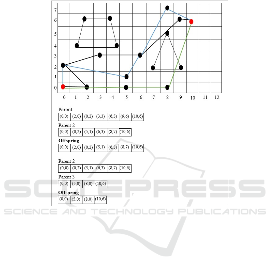
Figure 2: Intelligent crossover operator.
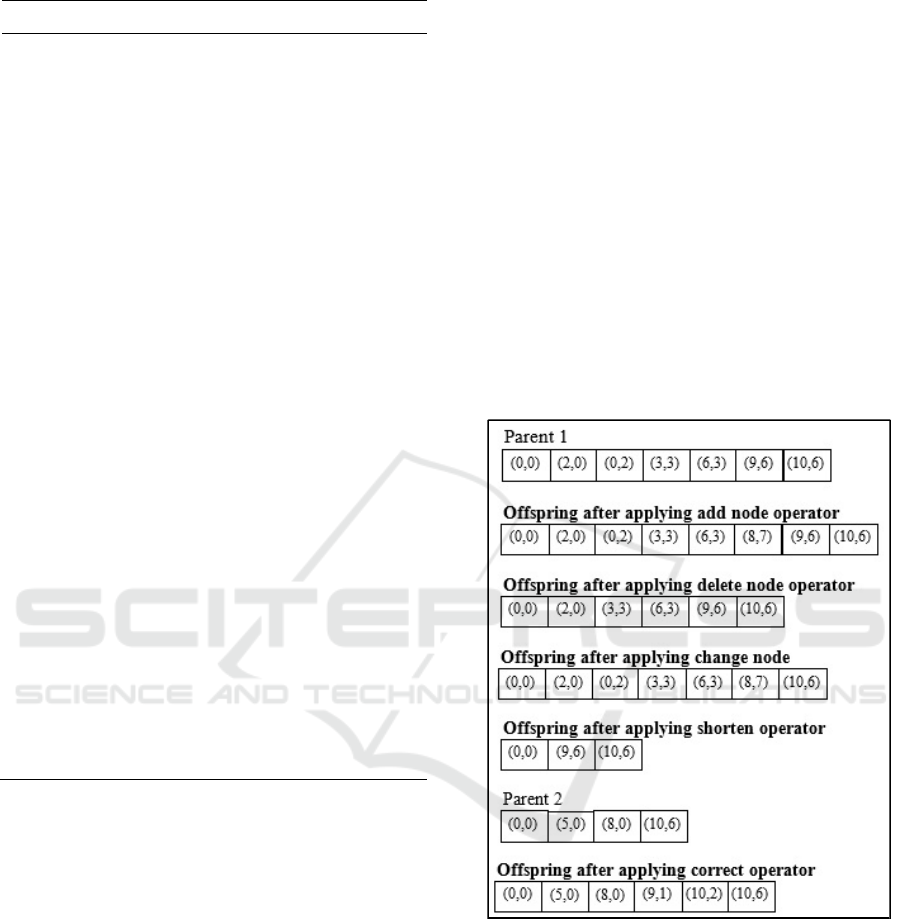
3.2.5 Mutation Operators
The mutation operator is primarily responsible for
giving GA the required diversity to explore the
entire solution space and prevent the population
from being stuck in a local optimum. In this paper,
we use five types of mutation operators:
a. Add Node: selects a random feasible cell
from the environment and adds it to the path
in a random index.
b. Delete Node: selects a random node from the
path and deletes it.
c. Change Node: selects a random node from
the path and exchanges its value with a
random feasible cell from the environment.
d. Shorten the Path: reduces unreasonable
curves in the path by deleting the intermediate
nodes between the nodes that have feasible
line segments.
e. Correct the Path: enhances the infeasible
path by correcting all infeasible parts, in
addition, it removes any duplicate nodes in the
path. To correct infeasible parts, the operator
uses the best first search algorithm (BFS)
based on Euclidean distance heuristic. BFS is
a simple heuristic search algorithm (Dudek
and Jenkin, 2010). We use it to help building
suboptimal path in fast time.
The mutation chooses one of these operators
randomly each time to generate new offspring.
Figure 3 shows an example for each operator, add
node, delete node, change node and shorten
operators are applied on parent 1, while correct
operator are applied on parent 2. The examples has
been taken from the represented map in figure 2.
3.2.6 Control Parameters
GA requires the various values of algorithm’s
parameters to be set, namely, population size,
crossover probability, mutation probability, and
stopping condition. These parameters have a great
impact on the performance and efficiency of the
algorithm; they affect the quality of the solution and
Enhanced Genetic Algorithm for Mobile Robot Path Planning in Static and Dynamic Environment
125
the search time.
a. Population Size: Research has indicated that
if the population size is too small, GA might
fail to reach a high-quality solution. On the
other hand, a large population size increases
the computational time of the GA (Al-Ajlan et
al., 2013). After performing some experiments
on the population size starting from 15 to 80,
the population size is set to 40, which can be
consider large enough to cover the
environment in which we work without
adding too much computational overhead.
b. Stopping Condition: After performing some
experiments on the stopping condition starting
from 50 to 200 iterations, the stopping criteria
of our GA are defined by 100 generations. We
chose this method to reduce the computational
time of the algorithm and give it enough time
to find the optimal solution.
c. Crossover and Mutation Probabilities: A
high crossover probability leads to the
generation of new individuals faster and
explores more solutions, but also it may leads
to disrupt the good solutions. Whereas, a high
mutation probability increases the diversity of
the population but risks the individuals
jumping over a solution to which they were
close and transforms the GA into a random
search. However, having excessively low
probabilities lead to solutions that become
stuck in local optima. Typically, the crossover
probability should range from 0.7 to 0.9,
whereas the mutation probability should range
from 0.01 to 0.1 (Al-Ajlan et al., 2013),
(Asteroth and Hagg, 2015). We will conduct
experiments to test different probability
values.
Figure 3: Examples on mutation operators.
3.3 Handling Dynamic Aspect
At the beginning, our GA tries to find the best path
based on the available static information. Then,
when change is detected, the GA seeks to manage
the dynamicity of the environment by using Memory
with Random Immigrants technique (MRI). This
technique has been selected because of its ability to
maintain population diversity, which is the key to
successful GA implementation for dynamic
problems and exploits useful information from
Algorithm 1: Intelligent Crossover Operator.
INPUT: chromosomes: parent1 and parent2, and node: goal
OUTPUT: new chromosome: child
BEGIN
1
2
3
4
5
6
7
8
9
10
11
12
13
14
15
16
17
18
19
20
21
22
23
24
25
26
27
28
29
30
31
32
child [1] = parent1[1]
n = 1
while (goal not reached)
x1 = find child [n] in parent1 and return the next node
x2 = find child [n] in parent2 and return the next node
if (x1 == null)
child [n+1] = x2
else
if (x2 == null)
child [n+1] = x1
else
f1= is(child [n], x1) line intersects with obstacles?
f2= is(child [n], x2) line intersects with obstacles?
if (f1 == false and f2 == true)
child [n+1] = x2
else
if (f1 == true and f2 == false)
child [n+1] = x1
else
d1=calculate Euclidean distance(child [n], x1)
+ calculate Euclidean distance(x1, goal)
d2=calculate Euclidean distance(child [n], x2)
+ calculate Euclidean distance(x2, goal)
if (d1 <= d2)
child [n+1] = x1
else
child [n+1] = x2
end if
end if
end if
end if
end if
n = n+1
end loop
END
ECTA 2016 - 8th International Conference on Evolutionary Computation Theory and Applications
126
previous phases (Elshamli et al., 2004). The memory
part is responsible for storing useful information
from the environment to be reused later in a new
environment. For every generation, we select the
best individuals from the population and add them to
the memory rather than the worst ones. Then, we use
all of its content to replace the worst individuals in
the population when the environment changed. The
random immigrant technique is a simple method to
address the convergence issue (Yang, 2008). It
maintains the diversity level of the population
through substituting a percentage of individuals in
the current population with new random ones when
the environment changed. Algorithm 2 shows how
the GA generates the new population based on the
MRI.
Algorithm 2: Memory with Random Immigrants.
INPUT: population p[], memory m[], start, goal,
and the number of random immigrants r
OUTPUT: new population g[]
BEGIN
1
2
3
4
5
edit start and goal nodes in all the paths in m[]
copy all the paths from m[] to g[]
generate r new random paths and add them to g[]
edit start and goal nodes in all the paths in p[]
copy (p[].size – r – m[].size) paths from p[] to g[]
END
4 PERFORMANCE
EVALUATION
At the beginning, we will test the algorithm with
different Crossover and Mutation probabilities to
study the effect of these two parameters on our GA.
Then, the static version of the algorithm will be
compared to A* (Tiwari et al., 2012), because it is
widely used in solving path planning problems due
to its optimality and completeness. In addition, it
will be compared to another efficient static GA
(Alajlan et al., 2016), (MGA). For dynamic
environments, we will compare the re-planning
method and the MRI to see the effect of using the
memory, as well as comparing the algorithm with
(Zhao and Gu, 2013) algorithm, (improved GA).
4.1 Experiment Setup
To test and evaluate the performance of our GA path
planner in different size environments, we designed
an object-oriented simulation model. We
implemented it by using C++ programming
language, and compiled it under Linux OS; Ubuntu
14.04 LTS. All the runs were conducted on a Dell
Venue 11i Pro device, which has an Intel Core i5
processor running at 1.6 GHz with 8 GB of RAM
and 104 GB of Disk.
In order to obtain a good analysis of the
algorithm, a set of benchmarks must be defined. The
benchmark set is composed of both simple and
difficult ones. The set consists of four different size
maps and different complexities (i.e. obstacle ratio).
The benchmarks were selected from (Sturtevant,
2012) and (Al-Ajlan et al., 2013). Figure 4 shows
the selected benchmarks. The dynamic environments
are simulated by introducing new obstacles during
the search process. Since the GA is a stochastic
technique, like all other metaheuristic techniques,
conclusions cannot be drawn from a single run. All
the results are based on the following: for each
configuration, ten runs are performed for the same
configuration. The best, average and worst cost, and
the average CPU time are registered for these runs.
4.2 Impact of GA Parameters
The aim of this section is to explore the impact of
mutation probability, crossover probability and the
proposed intelligent crossover operation on the GA
path planner. In order to do that, Map #2 was used.
4.2.1 Crossover Operator Impact
Table 1 demonstrates how Intelligent Crossover and
One-Point Crossover have impacted path cost and
CPU time. In order to calculate this, the generation
number was set to 100, population size to 40,
mutation probability to 0.01, and crossover
probability to 0.9. As can be clearly seen the two
types of crossover have different impacts on the
measured outcomes, where the Intelligent crossover
can find better path in much less time compared to
One-Point crossover.
Table 1: Crossover type impact.
Crossover
Type
Best
Path
Worst
Path
Average
Path
Average
Time
Intelligent
Crossover
71.562 102.123 86.1851 8.6251
One-Point
Crossover
72.198 164.201 110.126 14.4016
4.2.2 Crossover Probability
The impacts of the crossover probability (Intelligent
Crossover) on path cost and CPU time are shown in
Table 2. In order to calculate this, the generation
Enhanced Genetic Algorithm for Mobile Robot Path Planning in Static and Dynamic Environment
127
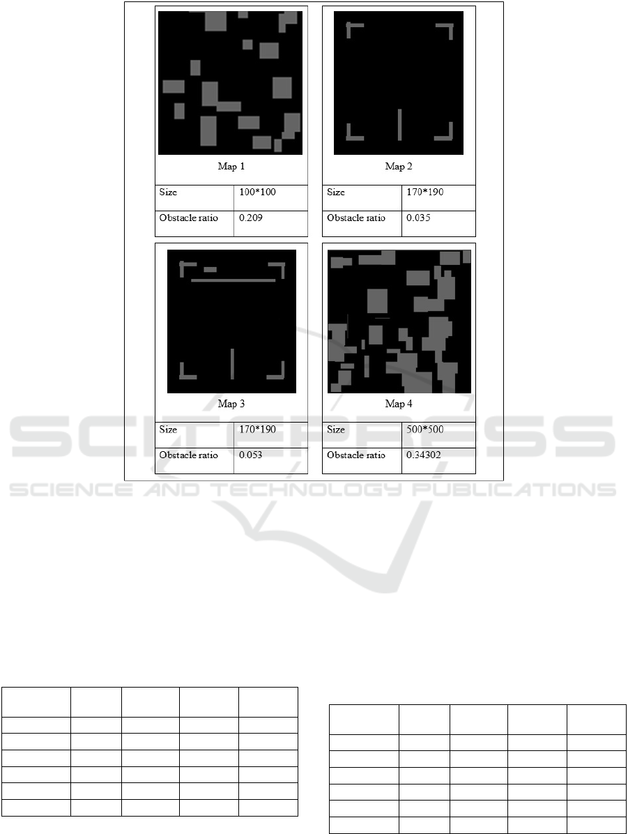
Figure 4: Benchmarks.
number was set to 100, population size to 40,
mutation probability to 0.01, and crossover
probability range from 0.5 to 1.0.
We can see that in table 2 increasing crossover
probability improves the average path cost but
equally increases execution time. Based on these
results, the most efficient crossover probability is
within the range of 0.7-0.9.
Table 2: Crossover probability impact.
Crossover
Probability
Best
Path
Worst
Path
Average
Path
Average
Time
0.5 69.044 146.474 94.52451 6.306106
0.6 71.428 148.066 99.11437 6.854905
0.7 70.201 130.608 97.18876 7.013214
0.8 72.639 110.968 88.08952 7.04423
0.9 71.562 121.339 86.18512 8.625075
1.0 74.062 180.799 125.0532 8.774862
4.2.3 Mutation Probability
The impact of mutation probability on path cost and
CPU time are shown in Table 3. In order to calculate
this, the generation number was set to 100,
population size to 40, crossover probability to 0.9
using Intelligent Crossover and mutation probability
range from 0.01 to 0.5. With an increase in mutation
probability, the average path cost improved but the
execution time increased alongside it. Therefore, the
most efficient mutation probability in terms of costs
and time is between 0.2-0.3.
Table 3: Mutation probability impact.
Mutation
Probability
Best
Path
Worst
Path
Average
Path
Average
Time
0.01 71.562 121.339 86.18512 8.625075
0.1 70.316 102.771 79.97139 7.377394
0.2 68.634 80.7936 73.47892 7.220681
0.3 69.170 73.2536 71.03801 7.987558
0.4 68.922 74.4373 70.88054 8.710724
0.5 68.719 70.7892 69.73331 8.77626
ECTA 2016 - 8th International Conference on Evolutionary Computation Theory and Applications
128
4.3 Performance Evaluation in Static
Environments
This section presents an evaluation of the
performance of the GA path planner in a static
environment focusing on path length as an indicator
of solution quality and execution time as an
indicator of the speed of the algorithm. This
performance is compared to A* and MGA. The GA
parameters, which produced the best results in the
previous section, were selected for all four
benchmarks: population size = 40, crossover
probability = 0.75, mutation probability = 0.3 and
number of iterations = 100. The start point is placed
at the topmost point on the left side, while goal point
is placed at the bottommost point on the right side in
order to increase the distance between them.
The results of all the four benchmarks for our
GA, A* and MGA can be seen in Table 4. For our
GA, we presented the best, worst and average path
costs and CPU times. For A* and MGA, as they
have similar results for all runs (best, worst and
average costs are all equal); we present only the
average path cost and the average CPU time.
Table 4 shows that our GA is able to find an
optimal or near optimal path, but as the complexity
and size of benchmarks is increased the gap between
the GA, A* and MGA also increases. In the last
benchmark, A* is better than GA 1.46 times. A*
finds the optimal path every time, but GA is an
incomplete method so it is not possible to be sure
that the GA and MGA paths are optimal. However,
as Table 4 shows, our GA was able on occasion to
find the shortest paths. This is because a grid-based
map used to represent the environment with
polygonal representation for the obstacles. This
approach means that the robot can move in any
direction with fewer detours than they are allowed in
the regular grid representation used by A* and
MGA, where robots can move in just eight
directions.
On other hand, the time gap between our GA and
A* and MGA decreases when the size of the
benchmarks increase. In large maps, GA
outperformed A* and MGA in terms of execution
time. For example, in the last benchmark, GA is
faster than A* 3.9 times. This is because our GA
uses random paths in the initial population and then
fix them later with the crossover and mutation
operators. This keeps the times low in most cases.
A* is a greedy approach, while MGA uses the
greedy approach to generate the initial population.
Both expands nodes exponentially with the depth of
the solution, which takes time during large
problems. In fact, MGA failed to complete the final
benchmark after 10 hours of trying, and overall it
took longer time to solve large problems.
4.4 Performance Evaluation in
Dynamic Environments
Here we tested the algorithms by using the first two
benchmarks. Again, the start and goal points were
chosen in the top left and bottom right cells. To
create a dynamic environment, user-defined
obstacles were introduced during each run in such a
way that they affect the best path produced in the
static mode.
4.4.1 Re-planning Vs Memory with Random
Immigrants
Two techniques were used to manage the dynamic
obstacles, MRI and re-planning. These were
compared in order to study the effect of using the
memory when the environment changes. The same
GA parameters that produced the best average
values were used for each technique: population size
= 40, crossover probability = 0.75, mutation
probability = 0.3, and number of iterations = 100.
Table 5 demonstrates that the MRI technique is
more efficient than re-planning from the start
because the MRI uses promising potential solutions
to improve the new path. The re-planning method
also had a longer execution time because it
generated more random paths that need to be fixed,
and this consume much more time.
Table 4: Results of GA, A* and MGA for four static benchmarks.
Benchmark
GA
A* MGA
Best Path Worst Path Average Path Average Time
Average Path Average Time Average Path Average Time
1 130.265 135.246 133.0312 7.903324
131.865 1.72329 131.865 0.95037
2 264.734 294.393 275.2191 9.216908
269.061 77.59117 269.061 11.07575
3 263.331 297.479 281.0732 13.40991
270.819 62.12198 290 23.12085
4 857.16 1178.8 1035.997 918.0374
805.919 3579.913 Failed
Enhanced Genetic Algorithm for Mobile Robot Path Planning in Static and Dynamic Environment
129
Table 5: Results of MRI and re-planning techniques in dynamic environments.
Benchmark
GA (MRI)
GA (Re-planning)
Best Path Worst Path Average Path Average Time
Best Path
Worst Path Average Path
Average Time
1 142.107 148.899 144.6106 17.59538
143.069 186.14 148.8587 17.68738
2 267.143 311.728 288.8071 29.18556
272.45 309.196 296.01564 34.66139
Table 6: Results of MRI and Improved GA in dynamic environments.
Benchmark
GA (MRI)
Improved GA
Best Path Worst Path Average Path Average Time
Best Path
Worst Path Average Path
Average Time
1 142.107 148.899 144.6106 17.59538
150.409 171.498 158.6494 26.7439
2 267.143 311.728 288.8071 29.18556
271.647 300.694 281.0783 139.4874
4.4.2 Comparison in Dynamic Environment
This section presents a comparative study between
our GA and the improved GA (Zhao and Gu, 2013)
in dynamic environments. They are assessed in
terms of solution quality, measured as path length,
and algorithm speed, measured as execution time.
The results of the evaluation are shown in Table
6. Both GAs were able to find optimal or near
optimal paths, although it is not guaranteed that
these are optimal because GA is not a complete
method. In our GA, the path cost was on average
slightly better than in the improved GA as a result of
the various mutation and crossover operations, and
as Table 6 shows, our GA found slightly shorter
paths. Again, this is a result of using the grid-based
map representation with polygonal obstacle
representation. For the same reason, our GA also
had consistently much better execution times than
the improved GA. Our representation is better since
the sizes of individuals are much smaller than the
size of individuals of the classical grid
representation. Therefore, the GA operations could
be performed efficiently.
5 CONCLUSIONS
Path planning is the process of deciding how to
move from one point to another one with respect to
the objectives of the problem. It is a fundamental
problem to mobile robots. In this paper, we
addressed the problem of path planning for mobile
robots in static and dynamic environment. Our
motivation was the need of finding the best path
within acceptable time, and studying the impact of
using a genetic algorithm in solving the problem.
This paper introduced a GA approach for solving
mobile robot path planning problems in static and
dynamic environments. The planner uses a grid-
based map with polygonal representation for the
environment as the knowledge base. The developed
GA planner uses variable-length chromosomes for
the path encoding to reduce the memory usage. Part
of the initial population is generated completely
randomly, while the second part is generated by one-
point crossover to get a diverse population with
paths of various quality in fast time and ensure that
some paths intersected with others to help
performing the intelligent crossover in later stage.
The fitness function is used to integrate the
objectives of the problem. Our GA uses two
selection operators: Elitist Selection and Tournament
Selection. In addition, the algorithm uses a new
crossover operator called Intelligent Crossover,
whereas, for mutation operation, five types of
mutation operators have been used. Furthermore, our
GA manages the dynamicity of the environment by
using Memory with Random Immigrants technique.
The GA was implemented by using C++
programming language and tested with four
benchmarks. We studied the impact of the crossover
operator, mutation and crossover probabilities, in
addition to MRI and re-planning techniques. We
also compared its performance in a static
environment against the A* algorithm and MGA
(Alajlan et al., 2016), as well as compared the
performance in a dynamic environment against
Improved GA (Zhao and Gu, 2013). It has been
shown that our algorithm is able to generate an
optimal or near optimal solution with fast execution
time compared to the three algorithms, especially in
large problems. In fact, we can accept some gaps to
optimality for enhancing the computational
expenses, since in real robotics applications; it does
not disadvantage to find paths with slightly taller
lengths, if they can be found much faster.
For future work, we intend to enhance the GA to
manage more dynamicity aspects, such as avoiding
ECTA 2016 - 8th International Conference on Evolutionary Computation Theory and Applications
130

moving obstacles and tracking moving goals. In
addition to improve the GA parameters.
REFERENCES
Alajlan, M. et al., 2016. Global Robot Path Planning
Using GA for Lagre Grid Maps: Modelling,
Performance and Experimntation. in press.
Al-Ajlan, M. et al., 2013. Global Path Planning for
Mobile Robots in Large-Scale Grid Environments
using Genetic Algorithms. Sousse, Tunisia, s.n., pp. 1-
8.
Asteroth, A. and Hagg, A., 2015. How to Successfully
Apply Genetic Algorithms in Practice: Representation
and Parametrization. Madrid, Spain, s.n., pp. 1-6.
Chaari, I. et al., 2012. smartPATH: A hybrid ACO-GA
Algorithm for Robot Path Planning. Brisbane,
Australia: IEEE Congress on Evolutionary
Computation.
Dudek, G. and Jenkin, M., 2010. Computational
Principles of Mobile Robotics. s.l.:Cambridge
University Press.
Elshamli, A., Abdullah, H. and Areibi, S., 2004. Mobile
Robots Path Planning Optimization in Static and
Dynamic Environments. Canda: Master thesis, The
University of Guelph.
Hussein, A. et al., 2012. Metaheuristic Optimization
Approach to Mobile Robot Path Planning. Cairo,
Egypt, s.n., pp. 1-6.
Koryakovskiy, I., Hoai, N. X. and Lee, K. M., 2009. A
Genetic Algorithm with Local Map for Path Planning
in Dynamic Environments. Montreal, Canada, s.n., pp.
1859-1860.
Mahjoubi, H., Bahrami, F. and Lucas, C., 2006. Path
Planning in an Environment with Static and Dynamic
Obstacles Using Genetic Algorithm: A Simplified
Search Space Approach. Vancouver, Canada, s.n., pp.
2483-2489.
Masehian, E. and Sedighizadeh, D., 2007. Classic and
Heuristic Approaches in Robot Motion Planning – A
Chronological Review. International Journal of
Mechanical, Industrial Science and Engineering, 1(5),
pp. 13-18.
Miao, H., 2009. Robot path Planning in Dynamic
Environments Using A Simulated Annealing Based
Approach. Brisbane, Australia: Master thesis,
Queensland University of Technology.
O'Rourke, J., 1998. Computational Geometry in C. Second
ed. New York, USA: Cambridge University Press.
Reshamwala, A. and Vinchurkar, D. P., 2013. Robot Path
Planning using An Ant Colony Optimization
Approach: A Survey. International Journal of
Advanced Research in Artificial Intelligence, 2(3).
Russell, S. and Norvig, P., 2002. Artificial Intelligence: A
Modern Approach (2nd Edition). s.l.:Prentice Hall.
Shi, P. and Cui, Y., 2010. Dynamic Path Planning for
Mobile Robot Based on Genetic Algorithm in
Unknown Environment. Xuzhou, China, s.n., pp. 4325-
4329.
Sturtevant, N., 2012. Benchmarks for Grid-Based
Pathfinding. Transactions on Computational
Intelligence and AI in Games, 4(2), pp. 144-148.
Sunday, D., 2012. Inclusion of a Point in a Polygon.
[Online]
Available at: http://geomalgorithms.com/a03-
_inclusion.html
[Accessed 11 March 2015].
Tiwari, R., Shukla, A. and Kala, R., 2012. Intelligent
Planning for Mobile Robot Algorithmic Approaches.
s.l.:IGI Global.
Yang, S., 2008. Genetic Algorithms with Memory- and
Elitism-Based Immigrants in Dynamic Environments.
Evolutionary Computation, Fall, 16(3), pp. 385-416.
Yun, S. C., Parasuraman, S. and Ganapathy, V., 2011.
Dynamic Path Planning Algorithm in Mobile Robot
Navigation. Langkawi, Malaysia, s.n., pp. 364-369.
Zhao, Y. and Gu, J., 2013. Robot Path Planning Based on
Improved Genetic Algorithm. Shenzhen, China, s.n.,
pp. 2515-2522.
Zhu, Z., Wang, F., He, S. and Sun, Y., 2015. Global Path
Planning of Mobile Robots Using A Memetic
Algorithm. International Journal of Systems Science,
46(11), pp. 1982-1993.
Zou, X., Ge, B. and Sun, P., 2012. Improved Genetic
Algorithm for Dynamic Path Planning. International
Journal of Information and Computer Science, May,
1(2), pp. 16-20.
Enhanced Genetic Algorithm for Mobile Robot Path Planning in Static and Dynamic Environment
131
