Swing Leg Trajectory Optimization for a Humanoid Robot

Locomotion

Ramil Khusainov, Alexandr Klimchik and Evgeni Magid

Intelligent Robotic Systems Laboratory, Innopolis University, Innopolis City, Russian Federation

Keywords: Humanoids, Bipedal Walking, Swing Phase, Optimal Trajectory Planning, Dynamic Programming.

Abstract: The problem of walking trajectory optimisation for bipedal humanoid robots attracts many researchers

because of excessive interest to bipedal locomotion. The main focus is usually on robot dynamics and

trajectory planning for predefined walking primitives. In contrast to other works, our paper targets to obtain

optimal walking primitive for swing leg trajectory of bipedal humanoid robot walking. Optimal walking

primitives are obtained taking into account velocity and acceleration physical limitations of each joint and are

derived for different walking parameters such as step size and hip height. To obtain a desired time-optimal

trajectory dynamic programing approach is used. It is shown that a new trajectory is performed within a

shorter time comparing with commonly used locomotion trajectories for bipedal robots control. The results

allow us to assign walking parameters and corresponding walking primitive that maximize robot velocity for

predefined environment constraints.

1 INTRODUCTION

To create a robot that could successfully operate in

environments that were originally designed for

humans, research community addresses to human-

like robots also known as humanoids. The growing

interest in the development of humanoids has been

observed for more than several decades (Channon et

al., 1992; Goswami, 1999; Katić and Vukobratović,

2003). The objective of research community is to

create a robot, which will operate with a human or

instead of him/her in dynamic environments,

including offices, factories, private and public

compartments, and be able to help in performing

various operations originally adapted for a human as

an actor.

Bipedal walking is one of the most natural and

attractive types of humanoid locomotion, since

bipedal robots provide more potential and flexibility

to move through rugged terrains and complex

environments, which create considerable difficulties

for wheeled or tracked robots due to their limited

locomotion capacities. On the other hand, bipedal

robots are less stable and may fall down while

performing even simple activities in rather standard

for a human environment where we efficiently

operate on a daily basis. Therefore, bipedal

locomotion stability related research keeps attracting

many researchers nowadays in order to propose good

robot locomotion control algorithms and to prevent a

biped robot from falling down (Akhtaruzzaman and

Shafie, 2010, Escande et al., 2013).

Among the variety of open research questions in

humanoids, robot body motion gains significant

attention of research community (e.g., (Hofmann et

al., 2009, Ude et al., 2004)), since it has a direct

impact on robot dynamics and stability. Here, the key

interest of researchers is related to dynamics and

trajectory planning for predefined walking primitives

(Kajita et al., 2001). However, the leg trajectory

optimality in a swing phase - a state in which the lifted

leg has no contact with a supporting plane and swings

forward - has not been studied in details yet. Similar

problems arise in robotic manipulators, when time-

optimal trajectory for a particular technological task

should be obtained (Pashkevich et al., 2002). In

humanoids, researchers usually use predefined

smooth trajectories for swing foot motions, such as

cycloids or third order polynomials (Ha and Choi,

2007). Because during the walking process a swing

foot has a maximal Cartesian speed among all

humanoid limbs, leg joint limitations play a key role

in a humanoid robot overall walking speed. In our

paper we propose a simple and effective method for

searching of an optimal swing leg trajectory within

130

Khusainov, R., Klimchik, A. and Magid, E.

Swing Leg Trajectory Optimization for a Humanoid Robot Locomotion.

DOI: 10.5220/0006011401300141

In Proceedings of the 13th International Conference on Informatics in Control, Automation and Robotics (ICINCO 2016) - Volume 2, pages 130-141

ISBN: 978-989-758-198-4

physical joint limits using dynamic programming

approach. Optimality of the trajectory is estimated

with a step traveling time criterion and also takes into

account velocity and acceleration limits of leg joints.

The obtained walking primitives with different

walking parameters (hip height, step size and time)

are used further to obtain optimal desired walking

primitive with a maximal robot velocity for

predefined environment constraints.

2 PROBLEM STATEMENT

There exist numerous approaches that are used for

bipedal robot locomotion control such as Central

Pattern Generation (Khusainov et al., 2015, Righetti

and Auke Jan, 2006), Neural networks, rule based

algorithms (Wright and Jordanov, 2014), gradient

optimisation technique (Ratliff et al., 2009) and

others. One of the most challenging strategies is so-

called passive-walkers (Collins et al., 2005, Collins et

al., 2001), which in some cases could be controlled

by a single actuator (Hera et al., 2013). The pioneer

method in modelling of a bipedal robot walking and

the most popular one is an analytical approach, which

defines equations for the robot locomotion under

some constraints induced by humanoid stability. This

approach has been used since 1970, when Miomir

Vukobratović proposed a so-called Zero Moment

Point (ZMP) stability constraint (Vukobratović and

Stepanenko, 1973). Currently, ZMP controller based

walking is the most popular approach, which

generates target trajectory of a humanoid robot in a

way that ZMP lies inside support polygon

(Vukobratović and Borovac, 2004, Sardain and

Bessonnet, 2004). Here, ZMP is a specific point on a

moving surface, where superposition of contact and

inertia forces does not produce horizontal moment. In

practice, the robot remains in a stable configuration

only if ZMP remains inside of a support polygon

(Erbatur and Kurt, 2009). ZMP stability constraint

equations are used to determine trajectory of Center

of Mass (CoM) for the robot (Mitobe et al., 2000).

ZMP approach is also used for trajectory generation

based on Inverted Pendulum Model (Majima et al.,

1999, Khusainov et al., 2016b) and Preview Control

(Kajita et al., 2003, Park and Youm, 2007). In these

methods CoM trajectory is a result of analytical

solution of dynamic equations for minimisation of

ZMP error in feedback control.

To the best of our knowledge, all algorithms for

bipedal robot stable walking select motion of leg

joints, which determine a swing leg movement,

without considering optimality of a trajectory. For

example, for NAO robot locomotion Motoc et

al.(Motoc et al., 2014) use a cycloid trajectory to

generate smooth motion, which is characterized with

zero velocity at the beginning and at the end of the

motion. Rai and Tewari (Rai and Tewari, 2014) use a

polynomial interpolation to obtain a swing leg

trajectory, assuming that robot’s CoM movement is

given. These approaches do not take into account

joint constraints and obtained trajectories do not

satisfy optimality from energy consumption point of

view. Therefore, the calculated trajectories of a swing

leg may be unattainable in practice because of

velocity/acceleration/jerk limits in joints and thus

would lead to wrong foot positioning, i.e. desired and

real trajectories would have a weak correspondence.

As a result, positioning errors accumulate with each

new step, which is a critical issue for autonomous

robots without global positioning feedback.

Figure 1: Full-size humanoid AR-601M (left) and its

kinematic structure in Matlab/Simulink environment

(right).

For our research we use anthropomorphic robot

AR-601M (Fig. 1) with 41 active degrees of freedom

(DoF), although we currently involve only 12 joints

(6 in each pedipulator) in the walking process.

Inverted Pendulum Model (Majima et al., 1999) with

ZMP stability constraint is used to generate CoM

trajectory. Here, six DoF of the supporting leg are

fully defined by CoM movement. For straightforward

motion it is assumed that in a frontal plane a swing

leg is perpendicular to the ground (or support plane)

at each time instance, a swing foot is parallel to the

ground, and a hip height remains constant during the

locomotion. These assumptions arise from human

natural walk analysis (Gabbasov et al., 2015) and are

widely applied in experimental works for biped

locomotion (Yussof et al., 2008). Taking into account

that a desired trajectory of a swing leg lies in a sagittal

plane, all joint coordinates of the swing leg are

uniquely defined for any foot and hip locations. In

this case the optimal trajectory problem is reduced to

2DoF system. Thus, the swing leg could be

Swing Leg Trajectory Optimization for a Humanoid Robot Locomotion

131

represented as a simple two-link system with hip and

knee joints. The corresponding to AR-601M robot leg

parameters link lengths are equal to 280 mm each.

Since in our models robot’s body moves at a constant

speed, for simplicity, we ignore body movement and

we assume a fixed position of the hip joint. This

means that the considered problem is represented in a

moving coordinate system. The trajectory of the

swing leg (solid line), support leg placement (dashed

line) and model parameters are shown in Fig. 2.

hip

0.5

ma x

Hip

Knee

Figure 2: Step motion of the swing leg in sagittal plane.

The primary research problem can be formulated

as follows: for given start and end points of a swing

leg and hip location, find an optimal trajectory, which

minimizes a selected cost function. Moreover, joint

angular velocities and angular accelerations during

locomotion should not exceed their maximal values.

The secondary research problem could be formulated

as follows: for a given robot and predefined obstacles

(which could be stepped over by the robot), obtain

optimal walking primitive that maximizes robot

speed in a given environment.

3 OPTIMISATION CRITERIA

There are different approaches to define cost function

in optimal trajectory search problem. For example,

Nakamura et.al. in (Nakamura, 2004) minimized

energy consumption, which can be written in the

form:

ii i

τθ γτ









(1)

where

is joint i torque,



is joint i velocity,

an empirical constant. The first term in (1)

corresponds to mechanical work, which is performed

to move dynamic system. The second term

corresponds to heat emission in each joint due to

torque generation. It was shown, that optimal

trajectory which could be found in such a way well

agrees with experimental data of human locomotion.

Yet, while obtaining a swing leg trajectory, the

authors do not take into account maximum joint

velocity and acceleration limitations, which actually

provide critical constraints for a real robot. A selected

trajectory could be energy optimal in theory, but if the

robot’s motors could not supply required by such

trajectory torques, the physical robot will fail to

perform such trajectory (Khusainov et al., 2016b).

In practice, walking speed is one of the most

important performance measures for bipedal robots.

Walking speed could be unambiguously calculated,

while energy consumption calculation is not that

obvious as it depends on many factors; e.g., energy is

mainly consumed in supporting leg joints, since they

have much higher actuating torques than swing leg

joints (in our work only swing leg motion is

considered). In addition, energy consumption

strongly correlates with step time: the faster a swing

leg moves for a given step length, the lower is its

energy consumption. Therefore, minimization of

each step time is a critical issue to be considered, and

it is the core contribution of our paper. Step time can

be evaluated as

()

tVdS=



(2)

where V is a foot speed in Cartesian space and

dS is

the foot path. Time t is calculated numerically by

dividing the trajectory into a finite number of

intervals and further summing up over all intervals.

4 OPTIMAL TRAJECTORY

SEARCH ALGORITHM

Optimal path for a bipedal robot swing leg could be

found with regard to different optimization

techniques. For example, in (Nakamura, 2004) spline

genetic algorithm (GA) was used to determine joint

torques for several points on the trajectory, which

were further used to interpolate joint torques for

remaining trajectory points introducing third order

splines. The main drawback of this approach is the

fact that genetic algorithms in general are not efficient

in finding a global minimum for continues functions

with multiple local minima (Renders and Flasse,

1996). An alternative approach for 6 DoF

manipulator has been used by Tangpattanakul and

Artrit (Tangpattanakul and Artrit, 2009)who utilised

a heuristic optimization method to find optimal

trajectory with Harmony Search algorithm. The

ICINCO 2016 - 13th International Conference on Informatics in Control, Automation and Robotics

132

obtained trajectories were smooth and complied all

kinematic constraints (both for velocity and

acceleration). However, in this approach only 6 via-

points have been used along the trajectory, which

limited its utilisations because of potential problems

between via points.

To overcome the above mentions limitations, in

this study, an optimal path is calculated using

dynamic programming approach (Si et al., 2009). The

key idea of this approach is to divide a large problem

into sub-problems of lower dimensions

corresponding to a transition between two via points,

to solve each of these sub-problems once and to store

the solutions. Advantages of this method are

robustness and computational efficiency compared to

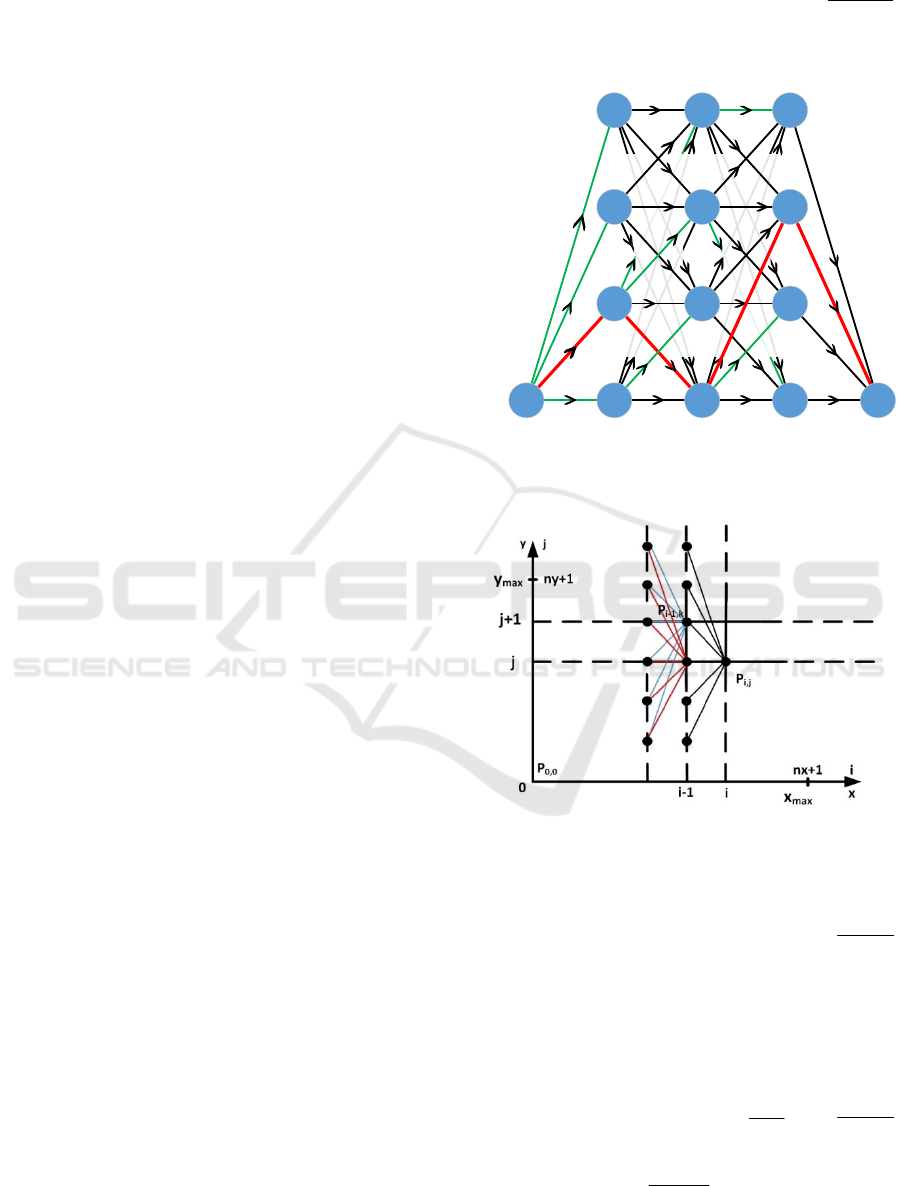
other methods. Illustration of this approach for a

simple case with three via points is shown in Fig. 3.

To find an optimal path from node (1,1) to node (5,1)

with a minimum total weight (time in the case of

optimisation walking trajectory) it is required to

examine all possible connections between these

points. Dynamic programing approach feature is that

via points are not specified exactly and can be

assigned to any node point of the row. Starting from

the left, for every node minimal total weight W is

computed and saved together with the node on the

previous layer, transition from which is optimal

(green lines in Fig. 3). For example, for node (2,2) the

minimal weight is 5 and the only transition from node

(1,1) is possible. For node (3, 1) minimal weight is 8

(5+3), which corresponds to transition from the node

(2,2). For node (3, 3) minimal weight is also 8 (5+3)

and corresponds to transition from the same node

(2,2) as for note (3, 1). For node (4, 3) minimal weight

is 12 (8+4), which corresponds to transition from the

node (3,1). Finally, we look at end point and find its

optimal transition. After that, to get the optimal path,

the optimal path from the last layer to the first layer is

constructed. For the provided example the optimal

path corresponds to the following path (red bold line

in the Fig. 3): (5,1), (4,3), (3,1), (2,2), (1,1).

To transform optimal path search problem for a

bipedal robot from continues optimisation problem

into a directed graph it is required to assign evenly

distributed nodes

,ij

within the search space, which

cover all possible trajectory paths. Here, to cover all

leg locations in x and y coordinates, it is necessitated

to create a two dimensional grid with

n +

points in

x direction and

n +

points in y direction (see

Fig. 4). Since the foot trajectories are considered with

a certain defined height limit

max

and step length

max

, the desired search space size is equal to

max max

y×

area, which contains

n −

via points to

be assigned (a single via point per each

2: 1

xn=−

, while y locations are constrained by potentially

traversable by the robot obstacles only).

1234

START

W=4

K=1

W=9

K=2

W=12

K=3

W=16

K=3

W=12

K=4

W=9

K=1

W=5

K=1

W=8

K=1

W=9

K=1

W=9

K=1

W=8

K=2

W=8

K=2

W=12

K=1

Figure 3: A directed graph for optimal path selection using

dynamic programming approach.

Figure 4: Building directed graph in search area by creating

2D grid.

The algorithm for finding the optimal path works

as follows:

• For each node point

,ij

1i =

1, 1jny=+

calculate the weight (i.e., the cost), which

corresponds to the minimal time of the transition

to that node from the start point

0,0

. For each

node save the weight and joints angular

velocities at the end point of the corresponding

trajectory.

• For each node

,ij

where

2,inx=

1, 1jny=+

calculate the weight of transition from

1,ki

−

node, where

0, 1kny=+

. Find

min

, for which

Swing Leg Trajectory Optimization for a Humanoid Robot Locomotion

133

the sum of the calculated weight for a transition

from

min

,ki

and total weight of

min

,ki

node is

minimal. For each node

,ij

save

min

k , the total

weight and joints angular velocities, which are

calculated for the transition from

min

,ki

,ij

• For node

nx 1,0

(the end point) calculate the

weight of the transition from

nx,k

, where

0, 1kny=+

. Find

min

, for which the sum of the

calculated weight and the total weight of

min

nx,k

node is minimal.

• Obtain an optimal trajectory by tracking

backward k

min

values for each node:

min min

min

1, 1

,1,

0,0

...

nx nx

nx ny

nx k nx k

ppp

−

→→ →

→→

(3)

where

min

is the optimal track for

1, 1nx ny

node.

Since the transition time between two node points

is used as a cost function, it is required to calculate

minimal traveling time from node

1,ki

−

to node

,ij

taking into account velocity and acceleration limits.

First, joint angles’ increments are calculated for each

transition between two adjacent nodes. Then we mark

a joint as active if it has larger absolute value of

angular increment for a given transition. Without loss

of generality let’s assume that joint 1 is active and

joint 2 is passive. Assuming that an active joint for

each interval moves either with a constant speed or a

constant acceleration (depending whether it reaches

the maximum velocity on previous interval), the joint

movements could be described as follows:

() () () 2

0.5

ii i

tat

ϕω

Δ= +

(4)

() () ()iii

ωω

(5)

where

i=1 for an active joint and i=2 for a passive

joint,

Δ is an angular increment,

and

are

angular velocities at start and end of the interval

respectively,

a is an angular acceleration (assumed to

be constant within the interval) and t is a transition

time.

In order to describe all possible relations between

active joints on adjacent intervals, three different

cases for calculating transition time should be

considered:

Case 1: Maximal Velocity. If an absolute angular

velocity of an active joint in

1,ki

−

node is equal to

maximum value

max

and its sign is equal to the sign

of angular increment

Δ , then

(1)

max

=Δ

(1)

0a = ,

(1) (1)

ωω

. Substituting t into equations (4)

and (5) we obtain

(2)

a ,

(2)

. It should be emphasized

that if the sign of angular increment

Δ is opposite

to the current velocity sign at the interval beginning

than either Case 2 or Case 3 should be applied.

Case 2: Maximal Acceleration. If an absolute

angular velocity of an active joint in

1,ki

−

node is

below its maximum value

max

or its sign is opposite

to the sign of angular increment

, then we

substitute

(1)

into equation (2) with

(1) (1)

max

()asign a

=Δ

and solve the second order

equation with respect to

(1) (1) 2 (1) (1)

(1)

()2

ww a

−± + Δ

(6)

Next, we select the lower positive root of the above

equation and calculate

(1) (1) (1)

ωω

. If

(1)

less than or equal to

max

, than

(1)

a and

(1)

are equal

to the calculated values. Finally, we substitute

t into

equations (4)-(5) to obtain

(2)

a ,

(2)

Case 3: Reaching Maximal Velocity. If Case 1

condition is not satisfied and

(1)

in Case 2 is greater

than

max

, than

(1) (1)

max

()

sign

=Δ

(1) (1) (1)

2/( )

ϕωω

=Δ +

(1) (1) (1)

()/

ωω

=−

. We

substitute t into equation (4)-(5) to obtain

(2)

a ,

(2)

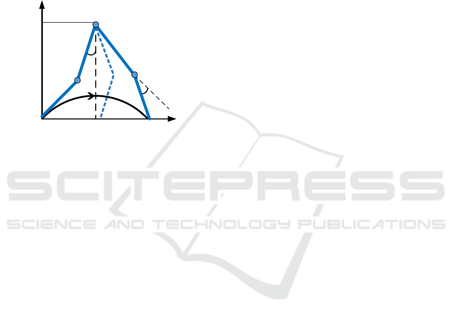
Figure 5 demonstrates all three cases which are

described above. For all cases we verify if the

calculated joint angular accelerations and velocities

are below their maximal values. If this condition

cannot be satisfied, such transition is excluded from a

possible path of the swing leg.

Figure 5: Three cases of angular velocity behavior: (1)

maximal velocity; (2) maximal acceleration; (3) reaching

maximal velocity

ICINCO 2016 - 13th International Conference on Informatics in Control, Automation and Robotics

134

5 SELECTING OPTIMAL

WALKING PRIMITIVE

It should be mentioned that for each given step length

and hip height a unique optimal walking primitive is

obtained. These primitives will have different weight

(traveling time) even in a case of an identical step

length but unequal hip heights. As a result, assigning

particular initial walking parameters affects robot

speed capacity. Therefore, considering different step

size and hip height it is possible to estimate robot’s

potential and to select the most appropriate primitive,

which ensures the best performance in terms of

robot’s speed. Another important issue that should be

also considered addresses particular characteristics of

the environment, i.e. presence of different obstacles

on the robot’s way, which could not be easily

circumambulated. To obtain an appropriate walking

primitive for negotiating a traversable obstacle (i.e.

stepping over such obstacle) the following algorithm

could be utilized.

Step 1: Specifying Constrains. Based on a

visible and technically traversable obstacle that

appears on the robot’s way, define feasible legs

locations for bipedal robot. The obstacle can be

approximated with rectangles and triangles that cover

all unreachable locations – as we address only 2D

case within a sagittal plane, only obstacle’s height and

length in robot’s walking direction are considered.

Step 2: Define Walking Parameter Limits.

Based on the robot geometry and current obstacle to

be negotiated, it is required to obtain reasonable

search intervals for step length and hip rising height,

i.e. their minimal and maximal values. Parameter

limits should be selected in such a way that at least

one trajectory with a continuous solution of inverse

kinematic problems exists between start and end

locations of a swing leg. Step size should be small

enough to detect extremum points.

Step 3: Finding Optimal Primitives for Each

Case.

For each combinations of a step length and a

hip rising height obtain optimal walking primitive and

traveling time using dynamic programming approach

presented in Section 4. If there is no solution of

inverse kinematic problem for at least one via point,

it is required either to decrease step size.

Step 4: Selection of an Optimal Walking

Primitive.

For each combination of walking

parameters estimate walking speed (in Cartesian

space) and select the optimal combination with regard

to a particular optimization criterion (i.e., the one with

the highest walking speed).

The above presented algorithm could be applied

for selecting optimal walking primitives for

humanoid robots with at least two DoFs within a

sagittal plane for each leg or could be further

extended for more DoF within a sagittal plane. It

gives a unique solution for the assigned initial

parameters of the robot and particular obstacle

properties, but the results are not being directly

scalable both between different robot models and

obstacles because of obstacles variety and physical

properties of various robots (link lengths, joint limits

for velocity and acceleration etc.). Thus, particularity

of robot kinematics always requires re-computing

optimal primitives for each specific model’s

parameters and each obstacle. Nevertheless, once

computed set of primitives for typical environment

conditions (i.e. different traversable obstacles) for a

particular robot model could be further applied for the

robot control for a whole set of robot motions.

6 SIMULATION RESULTS

The simulation of the algorithm was performed

within MATLAB/Simulink environment. The

acceleration and velocity limits were assigned to 1

rad/s

and 1 rad/s respectively for each joint. These

values correspond to technical characteristics of the

motors, which are used in AR-601M robot. First, let

us obtain optimal walking primitives for the fixed hip

rising height and step length and then compare results

with optimal parameters settings.

For the first case hip height was fixed to 0.5 m in

order to ensure optimal locomotion speed of the robot

based on our previous empirical studies (Khusainov

et al., 2016b, Khusainov et al., 2016a). According to

joint limits and link parameters we selected the robot

step length to be 0.4 m. For these parameters hip and

knee joint angles in their starting position were set to

0.1 and 0.55 rad correspondingly; at the end of the

trajectory (goal position) hip and knee joint angles

were set to -0.66 and 0.55 rad correspondingly. These

angles define

,ij

and

,ij

nodes.

Next, three different cases were analysed:

(i)

movement without any trajectory

constraints, i.e. in an ideal case without

velocity/acceleration limits the foot may

move straightforwardly from a start point to

an end point (Fig. 6);

(ii)

movement with 0.1 m barrier (with

negligible small size in the robot walking

direction) in the middle of the trajectory

(Fig. 7);

Swing Leg Trajectory Optimization for a Humanoid Robot Locomotion

135

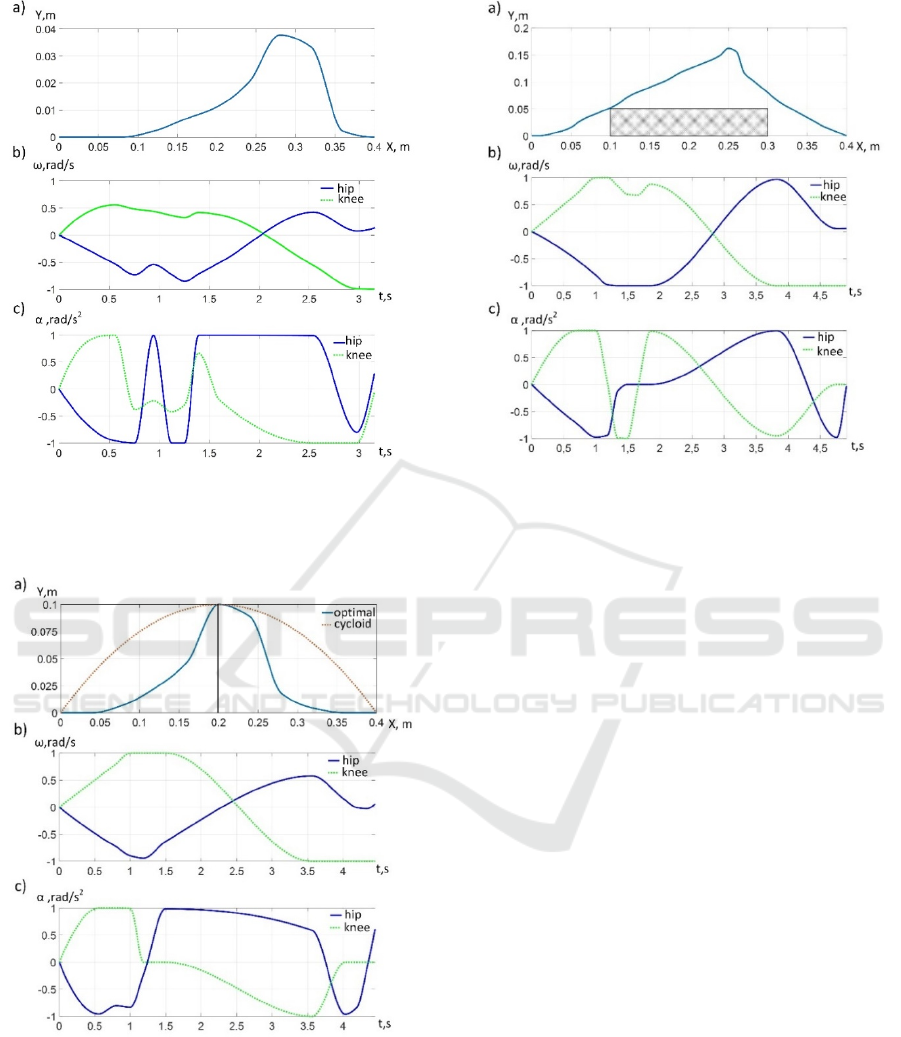
Figure 6: Optimal trajectory without obstacles for hip

height 0.5 m and step length 0.4 m: (a) foot trajectory in

Cartesian space; (b) angular velocity of joints; (c) angular

acceleration of joints.

Figure 7: Trajectories with 0.1 m barrier in the middle for

hip height 0.5 m and step length 0.4 m: (a) optimal foot

trajectory in Cartesian space and cycloid trajectory; (b)

angular velocity of joints; (c) angular acceleration of joints.

(i) movement with 0.05×0.2 m box barrier in

the middle (Fig. 8).

Figure 8: Optimal trajectory with 0.05×0.2 m box barrier in

the middle for hip height 0.5 m and step length 0.4 m: (a)

optimal foot trajectory in Cartesian space; (b) angular

velocity of joints; (c) angular acceleration of joints.

The results demonstrated that for all cases the

obtained Cartesian trajectories of a swing leg do not

correspond to the shortest path and differ from a

cycloid path, which is traditionally used in bipedal

robot locomotion control. To compare our results

with a cycloid path approach, we built the cycloid

trajectory for (ii) case and ensured the same travelling

time as for our optimal trajectory (Fig. 7a). The

corresponding angular velocities are presented in

Fig. 9. The simulation demonstrated that for the

cycloid trajectory, the knee angular velocity exceeds

maximum value and the accelerations at the

beginning and at the end of the trajectory are very

high. That means that in practice it is impossible to

perform such trajectory within the specified time. In

order to move along a cycloid trajectory, it is required

to scale (increase) travelling time according to the

velocity limits. Hence, the proposed algorithm

succeeds to suggest a foot trajectory with a shorter

time interval comparing to a typical cycloid

trajectory.

In the case without trajectory constraints, the foot

rises up to 0.04 m, which is caused by joint

velocity/acceleration limits. It is evident that travel

time in such case is minimum. The particularity of

this trajectory is that the joint velocity limits are not

reached (see Fig. 6b).

ICINCO 2016 - 13th International Conference on Informatics in Control, Automation and Robotics

136

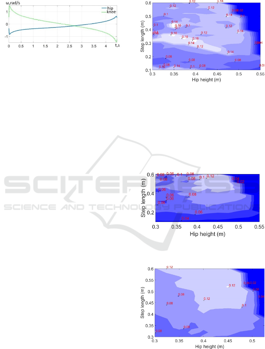
Figure 9: Angular velocities of joints for cycloid trajectory

movement with 0.1 m barrier, case of for hip height 0.5 m

and step length 0.4 m.

Barrier profile essentially effects optimal

trajectory (see Fig. 7a and Fig. 8a). Although the (ii)

case barrier is two times lower than for case (iii), the

height of the optimal trajectory for case (iii) and its

travel time are higher.

To compare efficiency of the obtained walking

primitives with conventional cycloids, the joint speed

and acceleration profiles have been obtained for

cycloids as well. It should be stressed, that these

profiles do not satisfy velocity and acceleration

limits, and to ensure such trajectory implementation

it is required to increase traveling time. In particular,

for free motions without obstacles the acceleration

limits have been exceeded by the factor 6, and to

remain within the limits traveling time should be over

10 s, which is twice higher that for the obtained

optimal trajectory. Another limitation of conventional

trajectory planning approach is its sensitivity to a

swing height and request to provide traveling time as

an input parameter. Our proposed approach does not

have these limitations and automatically estimates

minimal traveling time and an optimal swing leg

height.

Now, let us obtain optimal hip heights and step

length for all cases considered above and compare

robot performance. Speed maps for different step

length and hip height are presented in Fig. 10-12.

Here, lighter colour corresponds to higher speed and

are preferable for robot locomotion. It is shown that

Cartesian speed highly depends on the step length and

hip height and varies from one case to another. It is

also shown that optimal step parameters highly

depend on the size of the obstacle, which appears on

the robot path. In particular, for the case without

obstacles optimal settings are hip height of 0.4 m and

step length of 0.32 m, while for the case of box barrier

the optimal step length is much higher (0.52 m) and

hip height is almost the same (0.45 m).

Figure 10: Robot AR601M speed map for different step

length and hip height for the trajectory without obstacles.

Optimisation results are summarised in Table 1,

where for the three cases an optimal hip height, a step

length and a corresponding robot speed are given. For

comparison purposes it also contains robot speed for

the case of a fixed hip height and step length studied

above. It is shown that for the case of optimal hip and

step size parameters robot speed increases by 10-

23%, depending how far initial parameters were from

the optimal ones.

Figure 11: Robot AR601M speed map for different step

length and hip height for the trajectory with 0.1 m barrier in

the middle.

Figure 12: Robot AR601M speed map for different step

length and hip height for the trajectory with 0.05×0.2 m box

barrier in the middle.

Swing Leg Trajectory Optimization for a Humanoid Robot Locomotion

137

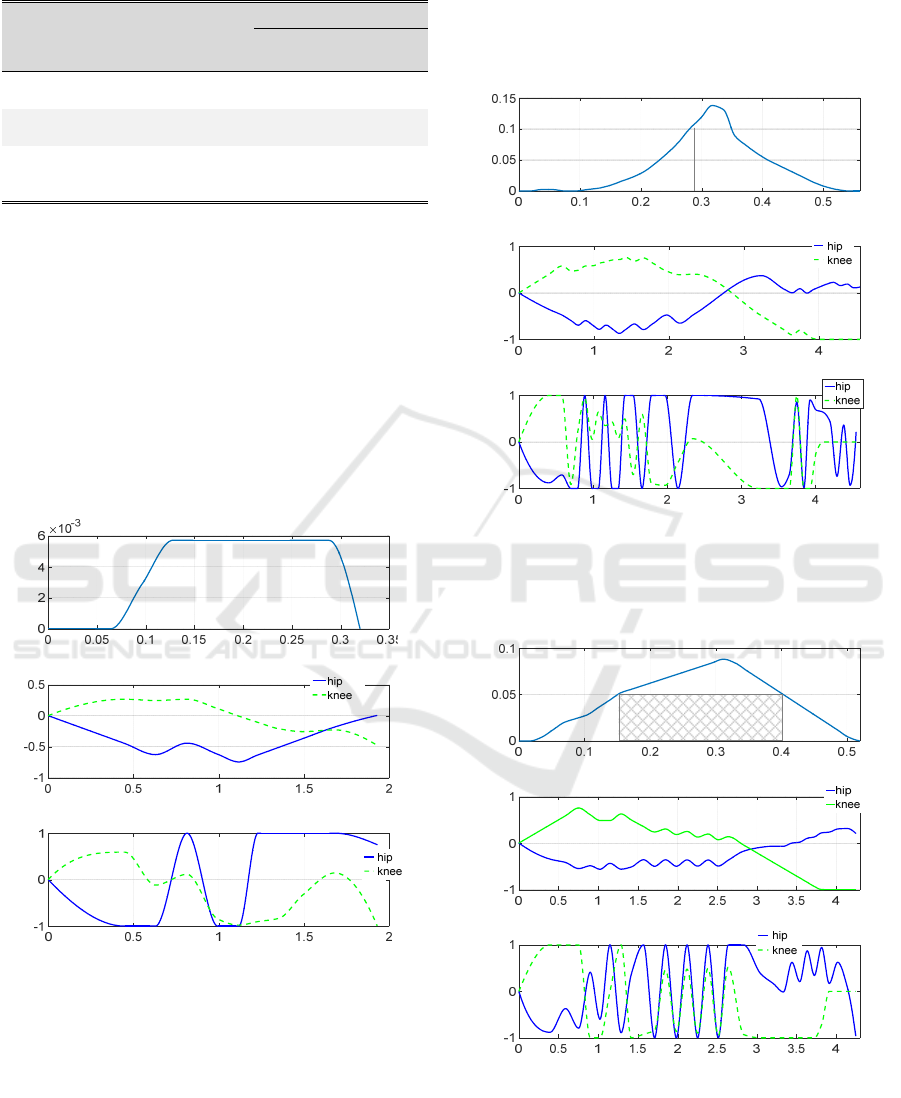
Table 1: Optimal walking parameters for locomotion of

bipedal humanoid robot AR-601M.

Case

Step

length

(m)

Hip

height

(m)

Speed (m/s)

Fixed

param.*

Optimal

param.**

(i) without

obstacles

0.32 0.40 0.13 0.16

(ii) with 0.1

m barrier

0.56

0.43 0.09 0.12

(iii) with

0.05×0.2 m

box barrier

0.52

0.45 0.11 0.12

*Fixed hip and step length parameters are 0.5 m and 0.4 m

respectively

**Optimal hip height and step length parameters

For comparison purposes Fig. 13-15 contain

walking primitives with joint velocities and

accelerations. It is shown that in the cases (ii) and (iii)

acceleration oscilations are essential (see Fig. 14c-

15c), which is mainly caused by problem

discretization and numerical calculation effects.

Nevertheless, these vibrations do not overcome

acceleration limits and will not affect robot

performance.

,/rad s

,ts

,/arad s

Figure 13: Optimal trajectory without obstacles for 0.4 m

hip height and 0.32 m step length: (a) foot trajectory in

Cartesian space; (b) angular velocity of joints; (c) angular

acceleration of joints.

A rather evident fact that for an optimal robot speed

without no obstacles, an optimal trajectory should be

close to the ground level was confirmed by simulation

results. It is clear that in practice such trajectory could

be hardly implemented (in fact, it is not possible to

have zero step height while locomotion), while it

demonstrates efficiency of the proposed approach.

With such moving primitive the robot can move with

0.16 m/s velocity instead of 0.13 that is maximal for

0.5 m hip height and 0.4 m step length. Similar

tendencies are observed for all considered cases.

,/rad s

,ts

,/arad s

Figure 14: Trajectories with 0.1 m barrier in the middle for

hip height 0.43 m and step length 0.56 m: (a) an optimal

foot trajectory in Cartesian space; (b) angular velocity of

joints; (c) angular acceleration of joints.

,/rad s

,ts

,/arad s

Figure 15: Optimal trajectory with 0.05×0.2 m box barrier

in the middle for hip height 0.45 m and step length0.52 m:

(a) an optimal foot trajectory in Cartesian space; (b) angular

velocity of joints; (c) angular acceleration of joints.

ICINCO 2016 - 13th International Conference on Informatics in Control, Automation and Robotics

138

7 DISCUSSIONS

In spite of numerous advantages, the proposed

walking trajectory optimization approach has several

apparent limitations, and the most significant one

among them is ignoring of dynamic and static effects

within optimization procedure. In fact, static effects

(compliance errors) are not critical for the trajectory

optimization since they are relatively small and could

be easily compensated by integrating a feedback

control from the feet force sensors. In this case the

main limitation for the moving primitive is avoiding

joint coordinates limits, which may not allow the

robot to compensate induced compliance errors. From

another side, if feedback control is not available

compliance errors should be computed using linear or

non-linear stiffness modelling (Klimchik et al., 2012,

Klimchik et al., 2014b) and control algorithm should

rely on the elasto-geometric model (Klimchik et al.,

2013, Klimchik et al., 2014a). It should be stressed

that stiffness parameters for real robot can be

obtained from the dedicated experimental study only

(Klimchik et al., 2015). So, statics effects the control

algorithm, but is not critical for optimization walking

primitives.

On the other side dynamic effects directly

influence robot stability (Majima et al., 1999, Mitobe

et al., 2000) and can be hardly compensated, since

this will directly affect walking primitive profile.

Since walking profile contains only foot coordinate,

humanoid torso and arms could be used to

additionally increase robot balance (Ude et al., 2004,

Yamaguchi et al., 1999). From another side,

integrating dynamic model into optimization

procedure may provide additional tool for trajectory

optimization. It may lead to faster robot movements

in the case when joint acceleration will be induced not

only because of actuation forces, but also by dynamic

forces. However, this approach essentially

complicates computations and may be hardly

implemented for robot control through joint angles

instead of demanded force level control. Besides,

swing leg does not contribute a lot in robot dynamics

since it does not effect robot body motion, which

mostly defining robot stability. In contrast, it is a

supporting leg (which is not considered in this work)

that mainly defines CoM trajectory and,

consequently, robot stability. From that point of view

supporting leg trajectory could be unambiguously

determined from stability condition while swing leg

coordinates are redundant variables that might be

optimised while step trajectory planning is proposed

in this work. So, the suggested in this paper approach

is a trade-off between a model complexity and

utilization of robot total capacities. In practice, to

avoid unpredictable robot behaviour, it is reasonable

not to use upper velocity/acceleration boundaries in

the optimization procedure since they may be higher

in real model because of a presence of dynamic forces

and errors in the model parameters.

The most essential limitation of the provided in

our paper results is related to kinematic constraints

induced to a hip location. It was strictly assumed that

the hip height remains the same along the trajectory,

while it is obvious that the best robot speed will be

achieved when the height varies along the trajectory.

In our approach, we separate swing and supporting

leg movements and consider only a swing leg

trajectory. Since a swing leg travels longer distances

in walking, its joints should apply higher speeds and

accelerations. Therefore, optimality due to kinematic

limits is more important for a swing leg. We consider

swing leg movement in coordinate system of a hip

where the hip is fixed. Another direction for

enhancing optimization efficiency is considering hip

speed as an additional optimization parameter, which

may vary from one via point to another. Providing

reasonable solutions of the above-mentioned

drawbacks and their integration into the optimization

algorithm will apparently lead to robot speed

increase. These issues will be addressed in details in

our future work.

8 CONCLUSIONS

In this paper we considered a problem of searching

optimal primitives for a swing leg trajectory, which

minimizes its travel time under joint angular velocity

and acceleration limits. Effective dynamic

programming approach was used to obtain a desired

optimal trajectory. It is shown that the obtained

optimal trajectory enables to decrease step time, i.e.

to increase robot speed compared to trajectories,

which had been traditionally used to control a swing

leg motion in bipedal robot locomotion. It is also

shown that the presented trajectory optimization

approach essentially increases speed of humanoid

robot AR-601M. The developed approach will be

further applied for optimization of a swing leg

trajectory with regard to a support leg and joint range

limits. Next, a set of optimal walking primitives will

be extended to the case of walking on the surface of

variable height (stairs and incline) as well as curved

paths that will bypass insurmountable obstacles and

walking in any direction. Besides, walking primitives

with variable hip height and hip speed will be

Swing Leg Trajectory Optimization for a Humanoid Robot Locomotion

139

considered as an objective for further optimization

algorithm enhancement.

ACKNOWLEDGEMENTS

This research has been supported by Russian Ministry

of Education and Science as a part of Scientific and

Technological Research and Development Program

of Russian Federation for 2014-2020 years (research

grant ID RFMEFI60914X0004) and by Android

Technics company, the industrial partner of the

research.

REFERENCES

Akhtaruzzaman, M. & Shafie, A. A. (2010) Evolution of

Humanoid Robot and contribution of various countries

in advancing the research and development of the

platform. Control Automation and Systems (ICCAS),

2010 International Conference on.

Channon, P., Hopkins, S. & Pham, D. (1992) Derivation of

optimal walking motions for a bipedal walking robot.

Robotica, 10 (02), 165-172.

Collins, S., Ruina, A., Tedrake, R. & Wisse, M. (2005)

Efficient Bipedal Robots Based on Passive-Dynamic

Walkers. Science, 307 (5712), 1082-1085.

Collins, S. H., Wisse, M. & Ruina, A. (2001) A three-

dimensional passive-dynamic walking robot with two

legs and knees. The International Journal of Robotics

Research, 20 (7), 607-615.

Erbatur, K. & Kurt, O. (2009) Natural ZMP Trajectories for

Biped Robot Reference Generation. IEEE Transactions

on Industrial Electronics, 56 (3), 835-845.

Escande, A., Kheddar, A. & Miossec, S. (2013) Planning

contact points for humanoid robots. Robotics and

Autonomous Systems, 61 (5), 428-442.

Gabbasov, B., Danilov, I., Afanasyev, I. & Magid, E.

(2015) Toward a human-like biped robot gait:

Biomechanical analysis of human locomotion recorded

by Kinect-based Motion Capture system. Mechatronics

and its Applications (ISMA), 2015 10th International

Symposium on.

Goswami, A. (1999) Postural Stability of Biped Robots and

the Foot-Rotation Indicator (FRI) Point. The

International Journal of Robotics Research, 18 (6),

523-533.

Ha, T. & Choi, C.-H. (2007) An effective trajectory

generation method for bipedal walking. Robotics and

Autonomous Systems, 55 (10), 795-810.

Hera, P. X. M. L., Shiriaev, A. S., Freidovich, L. B., Mettin,

U. & Gusev, S. V. (2013) Stable Walking Gaits for a

Three-Link Planar Biped Robot With One Actuator.

IEEE Transactions on Robotics, 29 (3), 589-601.

Hofmann, A., Popovic, M. & Herr, H. (2009) Exploiting

angular momentum to enhance bipedal center-of-mass

control. Robotics and Automation, 2009. ICRA '09.

IEEE International Conference on.

Kajita, S., Kanehiro, F., Kaneko, K., Fujiwara, K., Harada,

K., Yokoi, K. & Hirukawa, H. (2003) Biped walking

pattern generation by using preview control of zero-

moment point. Robotics and Automation, 2003.

Proceedings. ICRA '03. IEEE International Conference

on.

Kajita, S., Kanehiro, F., Kaneko, K., Yokoi, K. & Hirukawa,

H. (2001) The 3D linear inverted pendulum mode: a

simple modeling for a biped walking pattern generation.

Intelligent Robots and Systems, 2001. Proceedings. 2001

IEEE/RSJ International Conference on.

Katić, D. & Vukobratović, M. (2003) Survey of Intelligent

Control Techniques for Humanoid Robots. Journal of

Intelligent and Robotic Systems, 37 (2), 117-141.

Khusainov, R., Afanasyev, I. & Magid, E. (2016a)

Anthropomorphic robot modelling with virtual height

inverted pendulum approach in Simulink: step length

and period influence on walking stability. The 2016

International Conference on Artificial Life and

Robotics (ICAROB 2016). Japan.

Khusainov, R., Sagitov, A., Afanasyev, I. & Magid, E.

(2016b) Bipedal robot locomotion modelling with

virtual height inverted pendulum in Matlab-Simulink

and ROS-Gazebo environments. Journal of Robotics,

Networking and Artificial Life, 3 (1).

Khusainov, R., Shimchik, I., Afanasyev, I. & Magid, E.

(2015) Toward a human-like locomotion: Modelling

dynamically stable locomotion of an anthropomorphic

robot in simulink environment. Informatics in Control,

Automation and Robotics (ICINCO), 2015 12th

International Conference on.

Klimchik, A., Bondarenko, D., Pashkevich, A., Briot, S. &

Furet, B. (2014a) Compliance Error Compensation in

Robotic-Based Milling. In Ferrier, J.-L., Bernard, A.,

Gusikhin, O. & Madani, K. (Eds.) Informatics in

Control, Automation and Robotics: 9th International

Conference, ICINCO 2012 Rome, Italy, July 28-31,

2012 Revised Selected Papers. Cham, Springer

International Publishing.

Klimchik, A., Chablat, D. & Pashkevich, A. (2014b)

Stiffness modeling for perfect and non-perfect parallel

manipulators under internal and external loadings.

Mechanism and Machine Theory, 79, 1-28.

Klimchik, A., Furet, B., Caro, S. & Pashkevich, A. (2015)

Identification of the manipulator stiffness model

parameters in industrial environment. Mechanism and

Machine Theory, 90, 1-22.

Klimchik, A., Pashkevich, A., Caro, S. & Chablat, D.

(2012) Stiffness Matrix of Manipulators With Passive

Joints: Computational Aspects. IEEE Transactions on

Robotics, 28 (4), 955-958.

Klimchik, A., Pashkevich, A., Chablat, D. & Hovland, G.

(2013) Compliance error compensation technique for

parallel robots composed of non-perfect serial chains.

Robotics and Computer-Integrated Manufacturing, 29

(2), 385-393.

Majima, K., Miyazaki, T. & Ohishi, K. (1999) Dynamic

gait control of biped robot based on kinematics and

ICINCO 2016 - 13th International Conference on Informatics in Control, Automation and Robotics

140

motion description in Cartesian space. Electrical

Engineering in Japan, 129 (4), 96-104.

Mitobe, K., Capi, G. & Nasu, Y. (2000) Control of walking

robots based on manipulation of the zero moment point.

Robotica, 18 (06), 651-657.

Motoc, I. M., Sirlantzis, K., Spurgeon, S. & Lee, P. (2014)

Zero Moment Point/Inverted Pendulum-Based Walking

Algorithm for the NAO Robot. Emerging Security

Technologies (EST), 2014 Fifth International

Conference on.

Nakamura, M. (2004) Trajectory planning for a leg swing

during human walking. IEEE International Conference

on Systems, Man and Cybernetics.

Park, J. & Youm, Y. (2007) General ZMP Preview Control

for Bipedal Walking. Proceedings 2007 IEEE

International Conference on Robotics and Automation.

Pashkevich, A., Dolgui, A. & Chumakov, O. (2002)

Optimal control of robotic manipulator for laser cutting

applications. 15th Triennial World Congress of the

International Federation of Automatic Control.

Barcelona, SPAIN, 21th–26th July.

Rai, J. K. & Tewari, R. (2014) Quintic polynomial

trajectory of biped robot for human-like walking.

Communications, Control and Signal Processing

(ISCCSP), 2014 6th International Symposium on.

Ratliff, N., Zucker, M., Bagnell, J. A. & Srinivasa, S. (2009)

CHOMP: Gradient optimization techniques for

efficient motion planning. Robotics and Automation,

2009. ICRA '09. IEEE International Conference on.

Renders, J. M. & Flasse, S. P. (1996) Hybrid methods using

genetic algorithms for global optimization. IEEE

Transactions on Systems, Man, and Cybernetics, Part

B (Cybernetics), 26 (2), 243-258.

Righetti, L. & Auke Jan, I. (2006) Programmable central

pattern generators: an application to biped locomotion

control. Proceedings 2006 IEEE International

Conference on Robotics and Automation, 2006. ICRA

2006.

Sardain, P. & Bessonnet, G. (2004) Forces acting on a biped

robot. Center of pressure-zero moment point. IEEE

Transactions on Systems, Man, and Cybernetics - Part

A: Systems and Humans, 34 (5), 630-637.

Si, J., Yang, L., Chao, L., Jian, S. & Shengwei, M. (2009)

Approximate dynamic programming for continuous

state and control problems. Control and Automation,

2009. MED '09. 17th Mediterranean Conference on.

Tangpattanakul, P. & Artrit, P. (2009) Minimum-time

trajectory of robot manipulator using Harmony Search

algorithm. Electrical Engineering/Electronics,

Computer, Telecommunications and Information

Technology, 2009. ECTI-CON 2009. 6th International

Conference on.

Ude, A., Atkeson, C. G. & Riley, M. (2004) Programming

full-body movements for humanoid robots by

observation. Robotics and Autonomous Systems, 47 (2–

3), 93-108.

Vukobratović, M. & Borovac, B. (2004) Zero-moment

point — thirty five years of its life. International

Journal of Humanoid Robotics, 01 (01), 157-173.

Vukobratović, M. & Stepanenko, J. (1973) Mathematical

models of general anthropomorphic systems.

Mathematical Biosciences, 17 (3), 191-242.

Wright, J. & Jordanov, I. (2014) Intelligent Approaches in

Locomotion - A Review. Journal of Intelligent &

Robotic Systems, 80 (2), 255-277.

Yamaguchi, J., Soga, E., Inoue, S. & Takanishi, A. (1999)

Development of a bipedal humanoid robot-control

method of whole body cooperative dynamic biped

walking. Robotics and Automation, 1999. Proceedings.

1999 IEEE International Conference on.

Yussof, H., Ohka, M., Yamano, M. & Nasu, Y. (2008)

Analysis of Human-Inspired Biped Walk

Characteristics in a Prototype Humanoid Robot for

Improvement of Walking Speed. Modeling &

Simulation, 2008. AICMS 08. Second Asia

International Conference on.

Swing Leg Trajectory Optimization for a Humanoid Robot Locomotion

141