Soft Variable Structure Control in Sampled-Data Systems with

Saturating Input

Przemysław Ignaciuk and Michał Morawski

Institute of Information Technology, Lodz University of Technology, 215 Wólczańska St., 90-924 Łódź, Poland

Keywords: Nonlinear Control, Sampled-Data Systems, Variable Structure Control, Actuator Saturation.

Abstract: In the effort to achieve high convergence rate, at the same time avoiding implementation difficulties and

poor robustness of time-optimal controllers, the concept of soft Variable Structure Control (VSC) may be

applied. The classical formulation of soft VSC in continuous time domain assumes smooth switching among

an infinite number of controllers. Since nowadays control laws are implemented digitally, changing the

control structure is limited to sampling instances, which leads to quasi-soft VSC. The paper investigates

how the favourable characteristics of dynamic soft VSC can be extended to input-constrained systems with

finite sampling. The design procedure and stability analysis are conducted directly in discrete time domain.

The resulting nonlinear control law is synthesised into a form substantially different from its continuous-

time counterpart. However, smooth control action and fast convergence of continuous soft VSC is retained.

The properties of the obtained control system are formally proved and confirmed experimentally.

1 INTRODUCTION

A combination of two or more control structures

with switching logic results in new properties in thus

formed variable structure control (VSC) system. As

an example, one may consider two unstable systems

which, when joint by an appropriate switching

strategy, ensure asymptotic convergence to

equilibrium (Utkin, 1977). Depending on the design

requirements, the emphasis may be placed on

different aspects and properties of the VSC system.

When robustness is of primary importance (with

the quality of generated control signal a secondary

objective), a popular approach is to introduce a high-

gain switching element and create a sliding-mode

control system. Once the system enters the sliding

phase, any deviation from the prescribed manifold in

the state space is compensated, yielding insensitivity

to matched perturbations under ideal operating

conditions. In practice, physical limitations do not

permit achieving ideal sliding motion, yet high level

of robustness can be achieved. Special

considerations, however, need to be taken to

mitigate the impact of chattering – unfavourable

high-rate input oscillations that are destructive for

mechanical components and inefficient from the

point of energy budget (Lee and Utkin, 2007).

When a smooth control action becomes a

priority, a different class of VSC systems may be

considered. In particular, if high regulation rates are

desired, one can apply the concept of soft VSC

(Adamy and Flemming, 2004). Unlike sliding-mode

control that relies on infinitely fast switching

between a finite number of control configurations, in

soft VSC, an infinite number of cooperating

controllers is used in the effort to attain fast

convergence to equilibrium. The input signal

evolves smoothly within the range permitted by

constraints.

The soft VSC was originally developed for

continuous-time systems (Adamy and Flemming,

2004), and later explored also in continuous time

domain (Lens et al., 2011; Kefferpütz et al., 2013;

Liu et al., 2015). In now commonly applied digital

control realizations (Ignaciuk and Bartoszewicz,

2011; Ignaciuk and Morawski, 2014), however, it is

not possible to obtain switching at infinite rate. The

smoothness of control structure transitions in

discrete-time implementation of soft VSC is

restricted by the sequence of sampling instants. In

this paper, the design issues of soft variable structure

controllers for sampled-data systems are considered.

Although infinite switching rate among the control

structures is not possible, the obtained quasi-soft

VSC scheme ensures fast convergence to

Ignaciuk, P. and Morawski, M.

Soft Variable Structure Control in Sampled-Data Systems with Saturating Input.

DOI: 10.5220/0006001205450550

In Proceedings of the 13th International Conference on Informatics in Control, Automation and Robotics (ICINCO 2016) - Volume 1, pages 545-550

ISBN: 978-989-758-198-4

545

equilibrium with smoothly varying input signal. The

closed-loop stability and control signal constraints

are addressed explicitly and properties of the quasi-

soft VSC system are formally demonstrated within

discrete-time framework. The theoretical content is

supported by experimental study – stabilization of an

inverted pendulum-on-a-cart system.

2 PROBLEM SETTING

Let t = 0, 1, 2, ... denote subsequent time instants in

a system sampled with period T

. The system

dynamics are given by

[( 1) ] ( ) ( ),

sss

tT tT utT+= +xAxb

(1)

where x ∈ ℝ

is the state vector, u ∈ ℝ is the input

vector, A ∈ ℝ

n×n

and b ∈ ℝ

for n ∈ ℕ

. The initial

state x

= x(0) belongs to a bounded set X

. For

notational brevity, the independent variable tT

will

be written shortly as t in a latter part of the text.

The control input needs to obey the constraint

|| ,uu≤

(2)

> 0. It is assumed that the control system is

feasible, i.e. there exists control satisfying (2) that

can bring any x

∈ X

to 0. Equivalently, one may

consider only a (nonempty) set of points X

for

which control system (1)–(2) is stabilizable (Hu and

Lin, 2001).

3 SOFT VSC FOR

SAMPLED-DATA SYSTEMS

3.1 Soft VSC Concept

When the linear control u(t) = kx(t) with a fixed gain

k ∈ ℝ

1×n

is applied to system (1), the convergence

rate decreases as ||x||, ||⋅|| denoting the Euclidean

norm, approaches zero. In order to speed up the

performance, a nonlinear strategy, e.g. time-optimal

control, can be used. However, time-optimal

controllers, besides difficulties in obtaining

convenient form in sampled-data systems (Gao,

2004), imply sudden changes of the control input at

the extremity of allowed interval (2).

The idea behind soft VSC is to adjust the control

system dynamics by smoothly changing the control

structure so that high regulatory rate is maintained

throughout the whole movement from x

equilibrium. However, unlike continuous-time

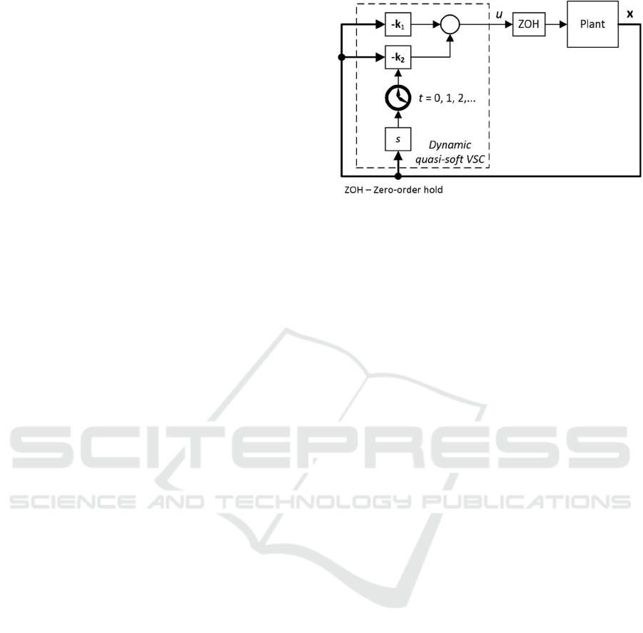
Figure 1: Dynamic soft VSC in sampled-data systems.

systems, discrete-time implementation does not

permit adapting the control structure infinitely fast.

The inherent characteristics of discrete-time control

call for special treatment to retain the desirable

properties of soft VSC systems.

3.2 Quasi-soft VSC

The analysed dynamic VSC system is illustrated in

Fig. 1. The control structure comprises two sub-

controllers and selection logic that governs the

overall gain adjustment. The input is determined as

() [ () ] (),ut st t=− +kkx

(3)

where k

, k

∈ ℝ

1×n

are the control gains and

s(t) ∈ ℝ is the selection variable used for gain

adaptation. The controller design amounts to

choosing suitable vectors k

and k

, and function

s(t).

The closed-loop system under control (3)

becomes

(1)[ () ]()

[()]()

tstt

st t

+= − −

=−

xAbkbkx

Abkx

(4)

with gain k

to be selected so that A

= A – bk

stable and good closed-loop performance is

achieved.

The system is required to have a single

(asymptotically) stable equilibrium point

⎡⎤ ⎡⎤

⎢⎥ ⎢⎥

⎣⎦ ⎣⎦

(5)

3.3 Selection Strategy

A possible choice of selection variable s(t) so that

(5) is the unique stable equilibrium for system (4) is

given in the following theorem.

ICINCO 2016 - 13th International Conference on Informatics in Control, Automation and Robotics

546

Theorem 1. If there exist positive definite

matrices P, Q, and R ∈ ℝ

n×n

satisfying

(),

−=− +APA P Q R

(6)

for A

= A – bk

, and the selection strategy is

chosen as

(1) (),

() () ()[ 2 ()

() ] ()

st rt

rt ws t t st

st t

=+ +

−

xR APbk

kbPbk x

(7)

with v > 0, 0 < w < 1, and R adjusted so that r(t) ≥ 0,

then (5) is the stable equilibrium of system (4).

Proof. Consider the Lyapunov function candidate

() () () ().

Vt t t vs t=+xPx

(8)

Since P is positive definite and v positive,

V(t) > 0 for t > 0 and V = 0 at equilibrium (5).

Therefore, in order for (8) to be a Lyapunov function

for system (4), the forward difference

() ( 1) ()Vt Vt VtΔ=+−

(9)

needs to be negative along the state trajectory.

Using (4) and (8), ΔV becomes

1212

12 2 1

() ( 1) ( 1) ( 1)

() () ()

()[()][()]()

(1) ()() ()

()[ ] () ( 1) ()

()[ () ()( )

()( ) ] ()

TT T

Vt t t vs t

ttvst

tst st t

vs t t t vs t

ttvstvst

tst st

st t

Δ=+ ++ +

−−

=− −

++− −

=−++−

+− −

xPx

x A bk P A bk x

xPx

xAPAPx

xAPbkbkPA

bk Pbk x

12 2 2

()[ ] () ( 1) ()

()[ 2() () ] ().

TT TT

ttvstvst

tst st t

=−++−

+− +

xAPAPx

xAPbkkbPbkx

(10)

Substituting (7) for s

(t + 1) in (10), yields

() ()[ ] () () ()

(1 ) ( ).

TT T

Vt t t t t

wvs t

Δ= − +

−−

xAPAPxxRx

(11)

Since v > 0 and 0 < w < 1, using assumption (6)

leads to

() () () (1 ) () 0.

Vt t t wvs tΔ=− −− <xQx

(12)

Consequently, since ΔV(t) < 0, V(t) given by (8) is a

Lyapunov function for system (4), and the system is

stable. 

Note that for a stable matrix A

(whose

eigenvalues can be moved into the open unit disc by

proper selection of vector k

), (6) represents a

Lyapunov equation with positive definite solution P

obtained for arbitrary positive definite matrix Q + R.

Thus, since the sum of positive definite matrices is

positive definite, one can always find positive

definite matrices P, Q, and R satisfying relation (6).

On the other hand, for sufficiently large R and v one

can guarantee that the expression under the square

root in (7) will be nonnegative, which results in a

feasible function s(t). Q can be arbitrary, e.g. an

identity matrix.

3.4 Actuator Saturation

The selection variable needs to be chosen in such a

way that the closed-loop system is stable, and input

constraint (2) is satisfied at all times. Directly from

(3), it follows that condition (2) is met whenever

01 20

[()],ustu−≤− + ≤kkx

(13)

which is equivalent to the pair of inequalities

01 01

( ) for 0,

( ) for 0.

−− −

≤≤ >

−−−

≤≤ <

kx kx

(14)

When x approaches the equilibrium thus formed

bounds extend to infinity. Therefore s should be

further limited as

|()|

ts≤

(15)

with s

being a positive constant. Combining (14)

and (15) one arrives at

() () ()

ssts≤≤xx

(16)

where

01 01

() , ,

⎧

−−+

≤

⎪

−+ +

⎪

=− <<

⎨

⎪

−− +

≥

⎪

⎩

kx kx

xkx

kx kx

(17)

and

Soft Variable Structure Control in Sampled-Data Systems with Saturating Input

547

01 01

() , ,

⎧

−− −−

≤

⎪

−− −

⎪

=<<

⎨

⎪

−−

≥

⎪

⎩

kx kx

xkx

kx kx

(18)

Theorem 2. If there exist positive definite

matrices P, Q, and R satisfying (6) with R and v

adjusted so that r(t) given by (7) is nonnegative, then

the selection strategy

(1) (,)(),

trrt

+= x (19)

with

()

,sgn[()](),

( , ) sgn[ ( )], ( ) sgn[ ( )] ( ),

()

,sgn[()] (),

st r s

rstsstrs

st r s

⎧

≤

⎪

=<<

⎨

⎪

≥

⎪

⎩

xx x

(20)

(x) and s

(x) given by (17) and (18), and

1, 0,

sgn( )

1, 0.

−≤

⎧

⎨

⎩

(21)

stabilises system (4) at equilibrium (5) while

upholding input constraint (2).

Proof. First, note that (20) makes s given by (19)

confined to interval (16), which is equivalent to the

constraint |u| ≤ u

Consider the Lyapunov function candidate

() () () (),

Vt t t s t

=+xPx

(22)

Since

P is positive definite and v positive,

V(t) > 0 for t > 0 and V = 0 at equilibrium (5). Using

(4) and (19), the forward difference

12 2 2

()

()[ ] () () ()

()[ 2 () () ] ()

()[ ] () () (),

TT TT

ttvrtst

tst st t

t t vwst st

=−+−

+− +

=−++−

xAPAPx

xAPbkkbPbkx

xAPAPRx

(23)

which after applying (6) becomes

() () () (1/ ) ().

Vt t t wvs t

Δ=− − −xQx

(24)

Since v > 0, for sufficiently small w > 0, ΔV(t) < 0,

and closed-loop system (4) with input constraint (2)

is Lyapunov stable. 

3.5 Convergence

It remains to be determined whether the control

system governed by the soft VSC strategy indeed

results in faster convergence than a linear scheme

with one controller. Note that

122 2

|( 1)|| ()|

()[ ] ().

()

TTTT

st st

wt t

vst

+= ×

++−

xAPbkkbPbkx

(25)

Assume |s| to be initially small (and disregard the

saturation effect). Then, the first term dominates the

quadratic form under the square root and |s| grows as

|( 1)||()| () ()

()

tstw tt

vs t

+≅ + xRx

(26)

providing increasingly faster decrease of V

according to (12). In consequence, the trajectory

approaches the origin at a faster rate than in the case

of static-gain linear control.

On the other hand, at the conclusion of the

regulation process, as x approaches zero,

|( 1)||()| .

tstw+≅ (27)

Since w < 1, |s| reduces to zero as well, effectively

leaving the system regulated by k

(which ensures

stable performance by definition).

4 EXPERIMENTAL STUDY

The controlled plant, illustrated in Fig. 1, reflects a

structurally unstable 4th-order inverted pendulum-

on-a-cart system. The plant parameters are as

follows: mass of the cart 0.768 [kg], mass of the

pendulum 0.064 [kg], moment of inertia (around the

centre of gravity) 0.00231 [kg⋅m

], and distance

between the pendulum gravity centre and the shaft

0.205 [m]. For the purpose of controller design a

linearized plant model is considered – the neglected

friction, nonlinearities, and actuator dynamics

constitute the plant uncertainty. Thus obtained

nominal plant dynamics are given by

ICINCO 2016 - 13th International Conference on Informatics in Control, Automation and Robotics

548

01 0 0 0

0 0 0.291 0 1.166

00 0 1 0

0 0 27.984 0 3.429

⎡⎤⎡⎤

⎢⎥⎢⎥

−

⎣⎦⎣⎦



(28)

where x = [x

... x

]

with x

– cart position, x

– cart

velocity, x

– pendulum angular position, and x

–

pendulum angular velocity. Input u is the motor

driving force adjusted through a PWM wave

generated from a microcontroller unit. The position

of the cart and pendulum is obtained from

incremental encoders with 1024 impulses per

rotation. The remaining state variables – the cart and

pendulum velocities – are determined from (noisy)

position measurements using a differentiating filter

with coefficients [1, –1]. Sampling time is set to

= 10 ms. The input constraint |u| ≤ 6.

Performance of three control strategies is

compared:

linear controller u(t) = – kx(t) with the gain

adjusted as k = [1.83, 2.58, 22.25, 4.12]. This

setting corresponds to the closed-loop

eigenvalues λ

∗

= 0.98 that yield the shortest

transient time without violating the input

constraint so that the system stabilizes in spite of

uncertainties;

fast controller with saturation limiting the input

to interval [–6, 6] [N] with the gain, set as

k = [38.52, 25.10, 81.76, 15.27], that

corresponds to the closed-loop eigenvalues

∗

= 0.94 in the linear region. The gain is selected

so that the fastest convergence permitted by

modelling inaccuracy and saturation nonlinearity

is achieved;

dynamic quasi-soft VSC (3) with selection

strategy (19): the control gains k

= [0.15, 0.40,

12.11, 1.91] (closed-loop eigenvalues λ

∗

= 0.985)

and k

= [12.19, 10.65, 46.69, 8.74] (closed-loop

eigenvalues λ

∗

= 0.955), s

= 100, v = 100,

w = 0.9, R = diag{0.2, 1, 0.2, 1}.

The cart is initially at rest with the pendulum

diverted from the upper unstable equilibrium by 30°

(which further strains the test owing to larger

inaccuracy in plant model linearization). The

objective is to drive the state to zero.

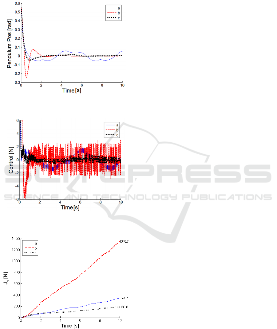
The system output (pendulum position) is plotted

in Fig. 3 and the corresponding input signal in

Fig. 4. All three controllers bring the output to the

vicinity of zero. As expected, the slowest

convergence is attained by the linear controller,

which also results in the largest limit cycle induced

by the nonlinearities of the physical plant. The

saturating and quasi-soft VSC strategies achieve

Figure 2: Experimental setup: A – inverted pendulum

mounted on cart E; B – motor; C – signal manipulation

device; D – microcontroller unit with the control logic.

similar convergence time with smaller overshoot

exhibited by the latter. The quasi-soft VSC shows

much improvement over the linear scheme in terms

of convergence, at the same time avoiding

oscillatory input generated by the saturating

controller. The smoothness of input signal quantified

through J

(t) =

(1) ()

ui ui

−

+−

∑

, is illustrated in

Fig. 5.

5 CONCLUSIONS

The paper investigates application of soft VSC

concept in sampled-data control systems with

saturating input. Unlike the classical continuous-

time formulation, the control action is adjusted at

finite intervals permitted by the sampling period,

which results in quasi-soft behaviour. The presented

design procedure, specific to discrete-time systems,

allows one to preserve the favourable properties of

continuous-time VSC. In particular, the quasi-soft

VSC combines the benefits of fast convergence and

smooth control signals, leading to an attractive

solution to be implemented in digital control systems

with magnitude-constrained inputs.

ACKNOWLEDGEMENTS

This work has been performed in the framework of

project no. 0156/IP2/2015/73, 2015–2017, under

“Iuventus Plus” program of the Polish Ministry of

Science and Higher Education. P. Ignaciuk holds the

Soft Variable Structure Control in Sampled-Data Systems with Saturating Input

549

Ministry Scholarship for Outstanding Young

Researchers.

Figure 3: Pendulum angular position: a) linear, b)

saturating, c) soft VSC strategy.

Figure 4:

Control input

a) linear, b) saturating, c) soft

VSC strategy.

Figure 5: Input s

moothness

a) linear, b) saturating, c)

soft VSC strategy.

REFERENCES

Adamy, J., Flemming, A. 2004. Soft variable-structure

controls: a survey. Automatica 40(11): 1821-1844.

Gao, Z. 2004. On discrete time optimal control: a closed-

form solution. In American Control Conference,

Boston, MA, USA, 52-58.

Hu, T., Lin, Z. 2001. Control Systems with Actuator

Saturation. Boston: Birkhäuser.

Ignaciuk, P., Bartoszewicz, A. 2011. Discrete-time

sliding-mode congestion control in multisource

communication networks with time-varying delay.

IEEE Transactions on Control Systems Technology

19(4): 852-867.

Ignaciuk, P., Morawski, M. 2014. Linear-quadratic

optimization in discrete-time control of dynamic plants

operated with delay over communication network. In

Mediterranean Conference on Control and

Automation, Palermo, Italy, 412-417.

Kefferpütz, K., Fischer, B., Adamy, J. 2013 A nonlinear

controller for input amplitude and rate constrained

linear systems. IEEE Transactions on Automatic

Control 58(10): 2693-2697.

Lee, H., Utkin, V.I. 2007. Chattering suppression methods

in sliding mode control systems. Annual Reviews in

Control 31(2): 179-188.

Lens, H., Adamy, J., Domont-Yankulova, D. 2011. A fast

nonlinear control method for linear systems with input

saturation. Automatica 47(4): 857-860.

Liu, Y., Kao, Y., Gu, S., Karimi, H.R. 2015. Soft variable

structure controller design for singular systems.

Journal of The Franklin Institute 352(4): 1613-1626.

Utkin, V.I. 1997. Variable structure systems with sliding

modes. IEEE Transactions on Automatic Control

22(2): 212-222.

ICINCO 2016 - 13th International Conference on Informatics in Control, Automation and Robotics

550