The Compression Algorithm of the S-Transform and Its Application

in MFCC

Zihao Cui

, Limei Xu

, Min Chen

, Jianwen Cui

and Yuzhuo Ren

Institute of Astronautics and Aeronautics, Center of Robotics, University of Electronic Science and Technology of China,

No.2006, Xiyuan Ave West Hi-Tech Zone, 611731, Chengdu, Sichuan, China

Institute of Disaster Prevention Yunnan, Kunming, China

Keywords: S-Transform, Compressing Algorithm, MFCC, Re-sampling.

Abstract: The S-Transform which is used in many fields, is better in the methods of time-frequency analysis. Although

the S-Transform improves the time-frequency analysis, it also increases the algorithm complexity, resulting

in rapidly increasing the computing time and needing more memory. Therefore, the S-Transform is difficult

to be applied for real-time procession of signal. Based on the characteristics that human being is insensitive

to the voice frequency resolution, in this paper, we propose a compressing algorithm of the S-transform.

Through re-sampling frequency, the algorithm decreases data size, the computing time and computer memory

usage in the S-transform. The application of the algorithm in MFCC analysis shows the results is reliable

under the condition of re-sampling frequency resolution

HzΔ< .

1 INTRODUCTION

The beginning of research on speech features was in

the 1930s (Cheng et al., 1996). Lendbergh and his

colleagues first conducted the research on the

personal speech features. After decade, many kinds of

coefficients about speech features were proposed,

including the most important one, Mel Frequency

Cepstral Coefficients (MFCC) (Davis et al., 1980).

The MFCC was put up based on the ability of

auditory feeling in 1980 by Davis and Mermelstein,

is better in speech recognition and has been widely

applied in the speech research. Since 1995,

computation of MFCC has been improved based on

time-frequency analysis and Neural Network (

Abdalla

et al., 2013).

In 1996, the S-Transform(ST) is proposed

(Stockwell et al. 1996), aiming at processing the

seismic wave in earthquake exploration. ST is the

expanding of Short Time Fourier Transform (STFT)

(Liu et al., 2000) and Wavelet Transform (WT) (Qian,

et al., 2008). ST is better than other methods (Chen et

al., 2006, Lin et al., 2013) in time-frequency

resolution. According to the previous research (Lin et

al., 2013), ST has a more straightforward relationship

with Fourier Transform comparing with WT and a

clear physical significance which transform

coefficients are invariant frequency (Vidakovic et

al.,1995). The well performance of ST leads to its

extensive use (Assous et al., 2006). However, ST

increases algorithm complexity (Brown et al., 2010),

needs more computing time and computer memory,

and that is less practical in MFCC while quick

response needed.

For reducing computation cost of ST, some

efficient algorithm of ST are put forward. Through

eliminating redundant data, Brown et al. (2010)

suggest a fast ST that improves ST efficiency, but its

frequency is different from general ST, so how to get

real frequency is a problem (Zhang, 2013).

Depending on the features of Power Quality

Disturbances,

Yi et al. (2009) proposed a incomplete

S-transform(IST) that also is efficient than general

ST, but IST only treats main frequency, so it can only

be applied in special situation.

Basing on the features that speech is wide

frequency band and most people can recognize

limited frequency band, we propose an efficient

algorithm of ST that replaces a small section in

frequency domain with a point in the section, the

method decreases computation cost of ST in MFCC,

and was called Compressing S transform (CST).

Cui, Z., Xu, L., Chen, M., Cui, J. and Ren, Y.

The Compression Algorithm of the S-Transform and Its Application in MFCC.

DOI: 10.5220/0005990505390544

In Proceedings of the 13th International Conference on Informatics in Control, Automation and Robotics (ICINCO 2016) - Volume 1, pages 539-544

ISBN: 978-989-758-198-4

539

2 S TRANSFORMATION AND ITS

IMPROVEMENT

2.1 S Transformation

ST of continuous time signal

()ht

can be represented

as (Stockwell et al., 1996)

() ()

()

,expexp2

fft

Sf ht iftdt

τπ

∞

−∞

−

=−−





















(1)

In this formula, t and

is the same parameters about

time, and f is the frequency.

Obviously the width of the window (the product

and the real exponential) will decrease with

increasing frequency. Because the narrowed integral

window for the different frequencies, it will expose

different resolution. It means that ST can do multi-

scale analysis. For (1), its Fourier transformation is

() ( ) ( )

{}

,()exp2Sf H fw f i d

τααπατα

∞

−∞

=++−



(2)

() ( )

() exp 2Hf ht iftdt

∞

−∞

=−



(3)

() ()( )

,,exp2Wf wtf itdt

απα

∞

−∞

=−



(4)

Here,

is the frequency after convolution.

2.2 The Compressing S Transform

Using the discrete version on (2) , we have

()

{}

S[ , ] [ ] [ , ]exp 2

kHkWk i

τααπατ

−



(5)

[]

()

[]exp 2

kht ikt

=−



(6)

[]

()

,[,]exp2

Wk wtk t

απα

=−



(7)

From (5), the algorithm complexity of ST is

(log)on n

larger than FFT

(log)on n

. The

memory need for ST is

()on

. Here

nFT=⋅

, T is

duration of speech signal and F

is the sample

frequency.

Table 1 is the running time and memory of ST for

actual speech signal that sample frequency is 14 KHz.

The table shows that run time and needed memory

will increase sharply with increasing duration of

speech. For example, 60 seconds speech needs nearly

5000 multiple run time and 3800 multiple memory

needed with 1 second speech signal.

Table 1: Computation Cost of ST.

Sample

Length（second）

Runs

(*10^9)

Similar

memory(GB)

1s 1.87 0.73

2s 8.03 2.92

10s 232.3 73.01

60s 9625.2 2628

Generally, the frequency range of speech is 20 Hz

to 20 kHz, and the human hearing is far more

sensitive to sound between 100Hz and 500Hz, and the

frequency resolution of the human hearing is about

1.8

HzΔ≈

. It means we are unable to receive the

information a speech that frequency is too high or too

low. Depending on the features of speech and human

hearing, this article re-samples frequency points of

ST to compress the amount of data in ST operation

within an acceptable range of error, and improves the

operation efficiency of ST. we call the ST with

compressing data size as the compressing algorithm

of ST or compressing ST, Abbreviated as CST.

Through re-sampling, CST does not need to process

all time-frequency data.

For a small enough section, the algorithm only

picks up the intermediate point of section to participate

in operation of ST. Setting parameter C as the

compression rate, Fs is the sample rate, N is the data

size before compression and T is signal duration, for

section

[

]

(C 1) / 2, (C 1) / 2

kk−− +−

, k

point will be

picked up, then after resample, data size of ST will

change from N to Nc, and frequency resolution will be

Fs Fs C

ffCC

NTFsT

Δ=Δ= = =

(8)

When replaced section is small, approximately we

have

[]

−

=−

≈



(9)

Then, we have

[] [][]

()

{}

S, , , exp2

CC C

kHCkWCk iC

τααπατ

−



(10)

[][]

()

,,exp2

WC k wtk iC t

απα

=−



(11)

here

is the re-sample value of

, and

compression rate C is

ICINCO 2016 - 13th International Conference on Informatics in Control, Automation and Robotics

540

(12)

From (10), the data size of ST will decrease C

times that will lower computation cost.

3 THE APPLICATION OF THE

COMPRESSED ST IN MFCC

MFCC is an analysis method on hearing system of

human beings. For a time-domain speech signal,

procedure of MFCC includes: pre-emphasis, framing,

windowing, then for each frame, its Fourier amplitude

spectrum will be filtered with Mel filter group, after

that, all the filter output will be done with logarithm,

Discrete Cosine Transform (DCT) and so on.

Following is the Mel filter

0<(1)

2( ( 1))

(1) ()

(( 1) ( 1))(() ( 1))

()

2( ( +1) )

() ( 1)

(( 1) ( 1))(() ( 1))

0(1)

kfm

mkfm

fm fm fm fm

fm k

fm k fm

fm fm fm fm

kfm

−





−−



−<≤

+− − − −





−



<≤ +



+− − − −





(13)

Here,

()

is the Mel filter group, m is the m

Mel

filter, f(m) is the centre frequency of m

Mel filter, k

is frequency.

3.1 MFCC with CST

For general MFCC, how to select the frame length of

speech signal and window are two problems that

influence results of MFCC. The frame length must be

short enough to meet short-time steady state, but is

not too short to ensure sufficient frequency resolution

for FT. It is difficult what the window function should

be selected for the different window function will

result in different MFCC. The application of ST in

MFCC can simultaneously resolve two problems of

general MFCC.

For speech time-history y(t), after pre-emphasis,

its time-frequency signal

(, )Yt f

can be got with ST.

Then faming

(, )Yt f

can be done in time domain

according to (15) and need not to do FT for every

fame.

[]



(15)

Here,

TF= 

is the point number. Therein,

[

]

,Yik

is the discrete

(, )Yt f

. For CST, replace N with N/C.

Every frame energy of y(t) is

[

]

[

]

,,EYik ik=









(16)

The frame energy through Mel filter group is

()

(, ) , ( )

im E ik H k

−

Ω=



(17)

For

(, )imΩ

, do logarithm, then compute the

cepstrum of DCT transform, finally we have

[]

2(21)

( , ) log ( , ) cos

mfcc i n Y i m

−









(18)

Here i is the i

frame, n is the spectral line,

(, )mfcc i n

is N-dimension characteristic vectors of MFCC.

3.2 Error Analysis

The application of CST in MFCC must cause the

distortion of MFCC feature vector. Simply, the

distortion can be expressed with the mean square

error (MSE) as

()

2,1

(,)

in in

DXY X Y x y

=− = −

⋅



(19)

Here,

(,)

is MSE about MFCC feature vector

Y, X with or without CST.

4 RESULT VERIFICATION OF

COMPRESSING ALGORITHM

4.1 Operation Efficiency

From (10), the computing time-consuming of CST is

N/2C times of Inverse FFT with the algorithm

complexity

( log )on n

. In FFT, split-radix FFT

(Johnson, et al., 2007) is a better method with

computational complexity (

4log 6 8NNN−+

). For

CST, its time complexity is

(log/)on n C

, space

complexity is

(/)on C

, and has

/CNN×

time-

frequency points，then its computational complexity

()

4log 6 8/CNNN−+

. So it can reduce run time and

memory as C times in ST.

Under the condition of Inter Core I7-4790

processor, DDR3 1866 16GB memory, 64-bit

MATLAB software, we processed some speech

signals with duration from 1s to 4s at interval of 0.2s.

For CST, its compression rates are set from 1 to 13 at

interval of 2. For each speech time-history, six tests

The Compression Algorithm of the S-Transform and Its Application in MFCC

541

are performed, and the average of memory

consumption and run time is computed.

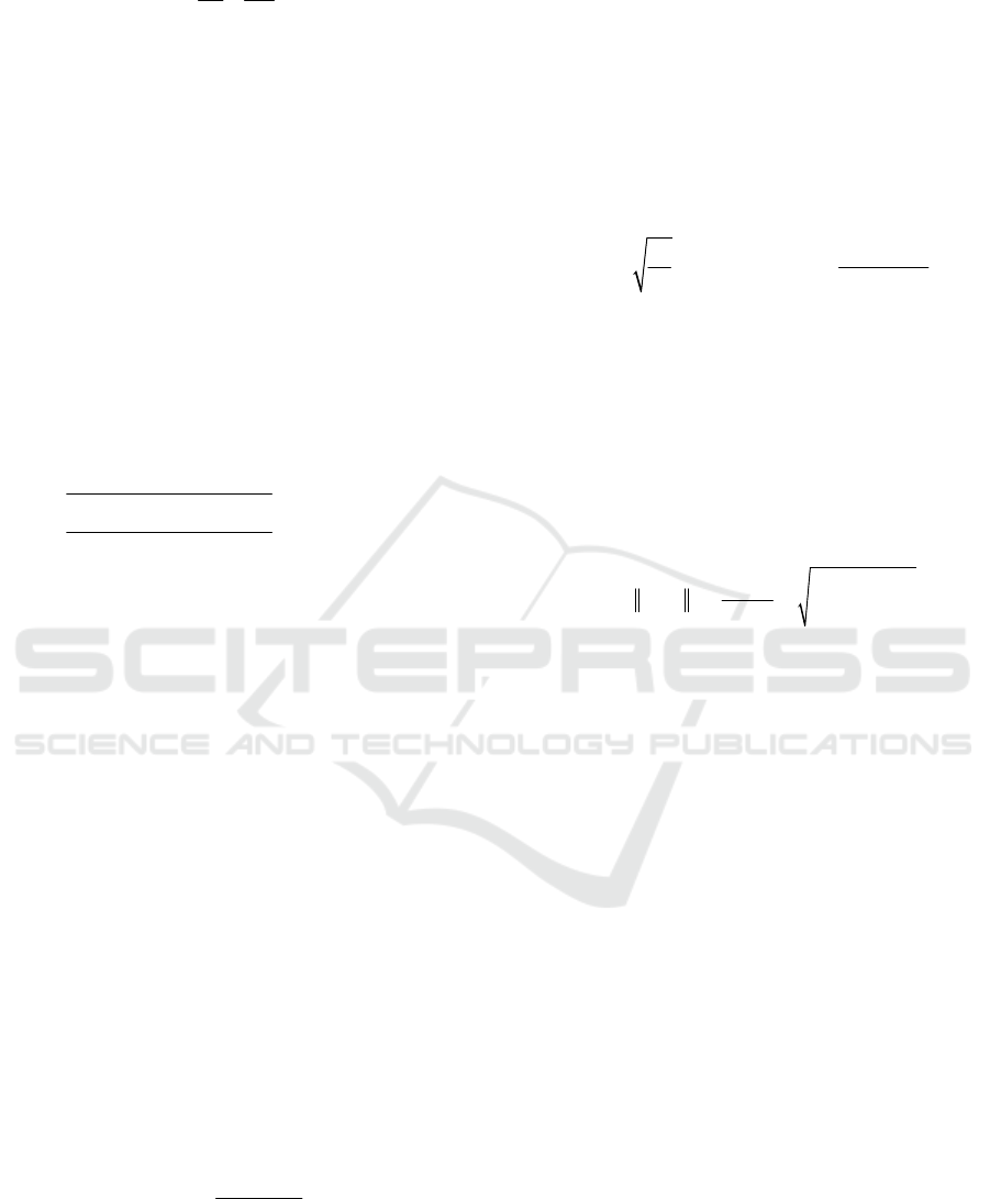
The figure 1 illustrates the relationship among run

time, compression rates and signal duration. The

figure 2 illustrates the relationship among memory,

compression rates and signal duration.

Figure 1: Relationship of Compression rate, sample time

and run-time (C is Compression rate that change from

1,3,5,7,9,11 to 13).

Figure 2: Relationship of Compression rate, sample time

and memory (C is Compression rate that change from

1,3,5,7,9,11 to 13).

When signal duration is longer than 4 seconds, the

memory is not enough to store the data and some data

must store in hard disk, the computation efficiency

drops rapidly and the run time increases to 1514s.

With the increasing compression, the needed memory

and the run time decrease significantly. For instance,

when the duration of speech is 3.6s, ST need 147s and

about 13GB memory, CST with triple compression

needs about 49s and 4.4GB memory which reduced

66% run time, and with thirteen compression needs

about 10.3s and 1GB which reduced 93% run time.

4.2 The Influencing of Compressing

Figure 3 is the time-frequency diagram of speech with

44.1KHz sampling frequency. In the figure 3, (a) is

uncompressing, (b) is 20 times compression. The

bottom of 3(a) and 3(b) is the time-history of speech,

the top is the time-frequency diagram, time-frequency

energy distribution in the figure is corresponding with

the time-history diagram. There is no significant

difference between two time-frequency diagrams.

(a) uncompressed time-frequency signal

(b) 20 times compression time-frequency signal

Figure 3: ST Time-Frequency analysis diagram.

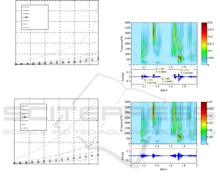
Figure 4 illustrates correlation of the MFCC

results computed from un-compression and

compression methods through linear regression

analysis. Two diagram show the results with 50 times

compression give the larger deviation that means that

error of results will increase with increasing

compression.

1 1.5 2 2.5 3 3.5

100

150

200

250

300

Signal Duration(s)

Run Time(s)

uncompressed

C=3

C=5

C=7

C=9

C=11

C=13

1 1.5 2 2.5 3 3.5

Signal Duration(s)

Memory(GB)

uncompressed

C=3

C=5

C=7

C=9

C=11

C=13

ICINCO 2016 - 13th International Conference on Informatics in Control, Automation and Robotics

542

(a) 50 times compression

(b) 20 times compression

Figure 4: Comparing the MFCC results with different

compression and uncompressing (horizontal ordinate is

uncompressed, vertical ordinate is compression).

Goodness of fit reflects level of similarity

between two vectors, defined as

()

 −

=−

 −

(20)

Here,

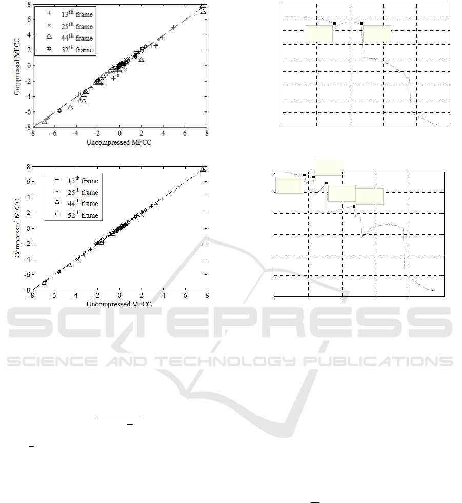
is the average of y, and figure 5 show that

the goodness of fit change with compression rate. In

figure 5, (a) and (b) are the results respectively with

male voice and female voice.

For figure 5, the signal duration is 0.38s that

eliminates zero energy points in speech. From

diagrams, the goodness of fit will decrease with the

compression rates increase. In the diagram, we can

find some important points, for male, these points are

C=31, 47, and for female, these points are C=18, 23,

31, 47. These points maybe reflect some features of

speech. From figure 5, we can get conclusion that the

larger compression can be used for male in the same

goodness of fit.

(a) The result with male voice

(b) The result with female voice

Figure 5: The Change of Goodness of Fit with Compression

ratio (in figure, horizontal ordinate is compression rate,

vertical ordinate is goodness of fit).

In speech recognition, a small difference of

MFCC will result in large recognition error, so in

order to ensure the reliability of the recognition

results, we limit that the goodness of fit is not smaller

than 0.99. Then for figure 5, we can find a key point

where the compression C=31, as long as the

compression is not larger than 31, either male or

female, the goodness of fit will is larger than 0.99. For

this key point, from (8), we have

=Δ <

(21)

That means, as long as re-sampling frequency

less than 82Hz, the results will be reliable.

5 CONCLUSIONS

ST is excellent in time-frequency analysis for high

resolution, energy concentration, and without cross

terms. The application of ST can resolve two key

0 20 40 60 80 100

0.96

0.965

0.97

0.975

0.98

0.985

0.99

0.995

1.005

X: 47

Y: 0.9976

X: 47

Y: 0.9976

X: 31

Y: 0.9977

Compression Rate(C)

Goodness of Fit(R

)

0 20 40 60 80 100

0.94

0.95

0.96

0.97

0.98

0.99

X: 18

Y: 0.9984

X: 23

Y: 0.9975

X: 31

Y: 0.9944

X: 47

Y: 0.9833

Goodness of Fit(R

)

Compression Rate(C)

The Compression Algorithm of the S-Transform and Its Application in MFCC

543

problems and improve accuracy in MFCC analysis,

but also be hindered due to the enormous operational

consumption.

Based on the features of human hearing and speech

is insensitive with speech signal resolution, the CST

re-sampling the frequency points in ST frequency

space to reduce data size in ST operation, effectively

reduces the run time and memory consumption of ST.

Applying CST in MFCC, the actual speech signal

analysis proves while re-sampling interval satisfies

HzΔ<

, the results of MFCC is reliable.

In this article, we set that the goodness of fit is not

smaller than 0.99, although it satisfies the reliability

of MFCC, it is at the expense of efficiency. So,

whether or not to adopt a smaller goodness value of

fit, when goodness of fit reduces, what phenomenon

will produce in recognition of speech based on

MFCC, and what a smallest goodness value of fit is

that can ensure in recognition of speech. Resolving

these problem will contribute to the effective

application of CST in MFCC.

ACKNOWLEDGEMENTS

We thank two anonymous reviewers for their helpful

comments. This research was supported by National

Nature Science Foundation of China (under the Grant

51578514), Yunnan, People Republic of China. It is

gratefully acknowledged for some fellows helping me

to collect the speech data.

REFERENCES

Abdalla M. I., H. M. Abobakr, T. S. Gaafar, 2013. DWT

and MFCCs based Feature Extraction Methods for

Isolated Word Recognition. International Journal of

Computer Applications, 69(20):21-25.

Assous S., A. Humeau, M. Tartas et al., 2006. S-transform

applied to laser doppler flowmetry reactive hyperemia

signals. IEEE Transactions on Biomedical

Engineering, 53(6):1032-1037.

Brown R. A., M. L. Lauzon, R. A, Frayne, 2010. General

description of linear time-frequency transforms and

formulation of a fast, invertible transform that samples

the continuous S-transform spectrum nonredundantly.

Signal Processing IEEE Transactions on, 58(1): 281-

290.

Cheng F., Gao S., 1996. Speech recognition technology and

development. Telecommunication Science, 12(10):54-

57. (in Chinese).

Chen Y. H., Yang C. C., Cao Q. F., 2006. Parameter

Estimation of Power Quality Disturbances Using

Modified Incomplete S-Transform. Progress in

Geophsics, 21(4):1180 ~ 1185(in Chinese).

Davis, S. B., Mermelstein P., 1980. Comparison of

Parametric Representations for Monosyllabic Word

Recognition in Continuously Spoken Sentences. In

IEEE Transactions on Acoustics, Speech, and Signal

Processing, 28(4):357-366.

Johnson. S. G. and M. Frigo, 2007. A modified split-radix

FFT with fewer arithmetic operations. IEEE Trans.

Signal Processing, 55(1):111-119.

Lin Y., Xu X., Li B., Pang J., 2013. Time-frequency

Analysis Based on the S-transform. International

Journal of Signal Processing, Image Processing and

Pattern Recognition 6(5) :245-254.

Qian K., Wang H., Gao W., 2008. Windowed Fourier

transform for fringe pattern analysis: theoretical

analysis. Applied Optics, 47(29):5408-5412.

Stockwell R. G., Mansinha L., Lowe R. P., 1996.

Localization of the complex spectrum: The S transform.

IEEE Trans. on Signal Processing, 44(4):998-1001.

Yi J. L., Peng J. C., Tan H. S., 2009. Detection method of

power quality disturbances using incomplete S-

transform. High Voltage Engineering, 35(10): 2562-

2567(in Chinese).

Vidakovic, B., P. Müller, 1995. An introduction to

wavelets. Computational Science & Engineering IEEE,

2(2):50-61.

Zhang Z., 2013. Application of Fast S-Transform in Power

Quality Analysis. Power System Technology,

37(5):1285-1290.(In Chinese).

Liu M., etc. 2000. Based on DWT and perception of voice

frequency domain filtering feature parameters. Circuits

and Systems, 5(1): 21-25. (in Chinese).

ICINCO 2016 - 13th International Conference on Informatics in Control, Automation and Robotics

544