Efficient Deployment of Energy-constrained Unmanned Aerial Vehicles
in 3-dimensional Space
Hunsue Lee, Junghyun Oh, Jaedo Jeon and Beomhee Lee
Department of Electrical and Computer Engineering, Seoul National University, Seoul, Republic of Korea
Keywords:
Multi-robot Path Planning, Unmanned Aerial Vehicle, Deployment, Energy Constraint.
Abstract:
In this paper, we present an efficient approach to deployment for unmanned aerial vehicles (UAVs). For a
number of scattered tasks, we aim to minimize the duration of time that all UAVs reach their task locations.
In our previous work, we suggested the collaborative deployment algorithm for mobile robots using a carrier
robot which transports and deploys the mobile robots. However, the method worked only in 2-dimensional
plane where UAV could not be applied. Therefore, this paper extends the previous work on 3-dimensional
space and gives the relevant algorithm. Finally, we presents the feasibility of the proposed algorithm by
simulation results.
1 INTRODUCTION
As unmanned aerial vehicle (UAV) is widely used,
a number of recent study is putting effort into the
development of UAV systems in robotics. The ad-
vantages of using UAV platform are that the UAV is
suitable for large scale operation such as exploration
(Sujit and Beard, 2008)(Luotsinen et al., 2004)(Su-
jit et al., 2009), simultaneous localization and map-
ping (SLAM) (Caballero et al., 2009), map-building
(Yang et al., 2005), search and rescue (Doherty and
Rudol, 2007)(Ryan and Hedrick, 2005), and surveil-
lance (Semsch et al., 2009).
On the other hand, the use of multi-robot system
(MRS) is unavoidable because the system can pro-
vide flexibility, fault-tolerance, robustness, and cost-
effectiveness (Yan et al., 2013). To use multiple
UAVs, the problem of multi-robot task allocation has
to be addressed. However, the general task allocation
problem is known to be nondeterministic polynomial
(NP) hard, meaning that optimal solutions cannot be
found quickly for large problems (Parker, 2008). The
deployment problem is also related with the task al-
location problem. Therefore, we need to reduce the
amount of computation so that the efficient path can
be generated within a finite time.
In this study, we use a team composed of two
kinds of heterogeneous robots, one carrier robot (CR)
and several UAVs, as shown in Figure 1. We as-
sume the CR has enough energy to complete a mis-
sion that is transporting and deploying the UAVs.
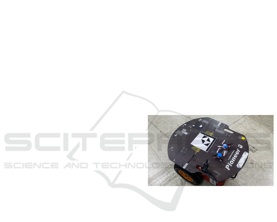
Figure 1: One Pioneer robot as the CR and two X12s as the
UAVs. The CR and the UAVs can be recognized and located
by using the artificial landmarks.
By using these two kinds of robots, the battery ex-
penditure of the UAV can be reduced and the total
travel distance of the UAV can be increased. There
are a few studies that use this cooperative strategy
(Wang et al., 2015)(Pei and Mutka, 2012)(Rybski
et al., 2000)(Saska et al., 2012). However, most of the
studies focuses on the mechanical implementation of
the system. Only a few existing studies discuss the
path planning problem (Mei et al., 2006). Finding the
optimal deployment path requires a lot of computa-
tion than the amount of computation for the traveling
salesman problem (TSP) (Lee et al., 2015b). To re-
duce the computation, we divided the tasks into sev-
eral clusters based on the geographical information of
the tasks. Then each optimal deployment location for
each cluster can be found. Finally, the deployment
locations are adjusted and merged into the solution.
446
Lee, H., Oh, J., Jeon, J. and Lee, B.
Efficient Deployment of Energy-constrained Unmanned Aerial Vehicles in 3-dimensional Space.
DOI: 10.5220/0005986904460451
In Proceedings of the 13th International Conference on Informatics in Control, Automation and Robotics (ICINCO 2016) - Volume 2, pages 446-451
ISBN: 978-989-758-198-4
Copyright
c
2016 by SCITEPRESS – Science and Technology Publications, Lda. All rights reserved
Although the solution does not guarantees the opti-
mality, the efficient path can be generated quickly.
The remainder of this paper is organized as fol-
lows. In Section 2, we give brief description of the
problem which has been presented in our previous
work. In the following section, we address the de-
ployment problem in 3-dimensional space. Then Sec-
tion 4 describes simulation results. Finally, in Section
5, conclusions are drawn, and areas for further work
are discussed.
2 PREVIOUS WORK
2.1 Problem Description
In the given environment, there are m tasks, n UAVs
where n ≥ m, and one CR. The CR’s velocity is v
C
,
constant acceleration and deceleration is a
C
, the max-
imum velocity is v
max
C
, and the rotating speed is w
C
.
The UAVs’ velocity is v
R
and its maximum traveling
distance is d
max
. Unloading of UAVs takes τ seconds.
Meanwhile, a task and its location is denoted by q and
v
q
respectively.
In the previous work (Lee et al., 2015b) (Lee et al.,
2015a), we have formulated the deployment problem
for scattered tasks whose objective is to finding the set
of optimal deployment points W
?
. Let T
i
is the dura-
tion of time that the CR moves to α-th deployment
location w
α
from the initial location, the CR deploys
i-th UAV, and the UAV moves to the target location
v
q
i
. Then T
i
is formulated as follows:
T
i
=
α
∑
k=1
f (w
k−1
,w
k
) + τ
+
kw
α
− v
q
i
k
v
R
(1)
By using (1), the objective function can be repre-
sented as follows:
W
?
= argminmax
W
[T
1
,T
2
,. ..,T
m
]
(2)
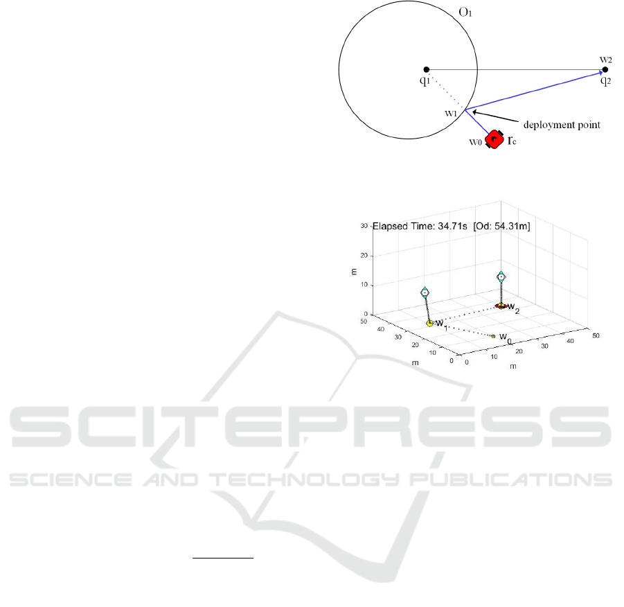
2.2 Path Planning Method
We also proposed a path planning algorithm of the
CR. If there are two tasks q
1
and q
2
as shown in Fig-
ure 2, we can always find the optimal deployment lo-
cation w
1
by finding the circle of Apollonius O
1
that
has given ratio of distances |v
max
C
|/|v
R
| to two given
points q
1
and q
2
.
Figure 2: Finding the optimal deployment location w
1
for
two given tasks, q
1
and q
2
.
Figure 3: Example of UAV deployment for two tasks in
50m × 50m × 30m space. We set v
max
C
= 10.0m/s,w
C
=
2.0rad/s, a
C
= 5.0m/s
2
,τ = 1.0s,v
R
= 2.0m/s.
3 UAV DEPLOYMENT IN 3D
SPACE
3.1 Optimal Deployment for Two Tasks
First we extends the simulation space into 3D. Fig-
ure 3 shows the example of UAV deployment for two
tasks in 3D space (W: 50m × D : 50m × H : 30m).
In the figure, blue diamonds represent the task loca-
tion, white circles represent the UAVs, yellow circles
represent the deployment locations, and the red rect-
angle represent the CR. As the CR cannot fly over
the ground, the coordinate of the CR is remained
in 2D plane. Unless the location of second task is
too far, the optimality of the deployment is achieved
by letting two UAVs reach their location simultane-
ously. However, the result in Figure 3 does not satisfy
the criterion as the previous algorithm works in 2D
plane. Therefore, the deployment location should be
adjusted.
Figure 4 describes how the optimal deployment
location can be obtained. Let z
1
and z
2
be the heights
of the tasks q
1
and q
2
respectively. If z
1
= 0 and
z
2
= 0, then the optimal deployment location w
1new
for q
0
1
and q
0
2
in Figure 4 is calculated by finding ∆d
Efficient Deployment of Energy-constrained Unmanned Aerial Vehicles in 3-dimensional Space
447
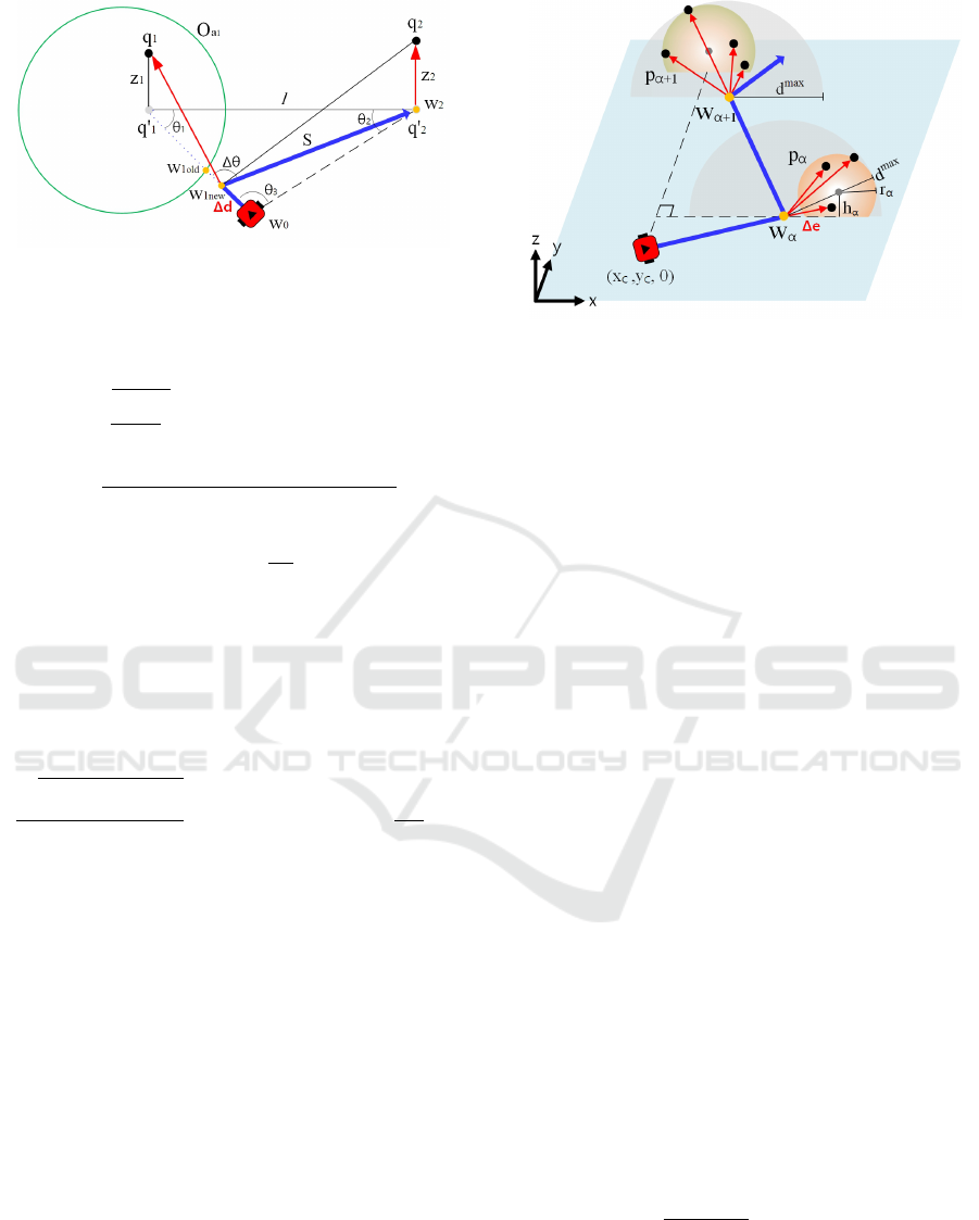
Figure 4: Finding the optimal deployment location w
1new
for two given tasks, q
1
and q
2
in 3D space.
as follows:
ξ − ∆d
v
R
= mv(w
1new
,w
2
) + τ (3)
where ξ = kw
0
q
0
1
k, mv(w
1new
,w
2
) is the duration of
CR’s moving time from w
1new
to w
2
, and:
S =
q
l
2
+ (ξ − ∆d)
2
− 2l(ξ − ∆d)cosθ
1
(4)
rt(θ
C
w
1new
) =
θ
3
+
∆d
ξ
· θ
2
/w
C
(5)
where rt(θ
C
w
1new
) is the function that returns the dura-
tion of rotating time at the deployment location w
1new
.
Expanding on this idea, we can find ∆d for q
1
and
q
2
by equalizing the durations that first UAV moves
from w
1new
to q
1
, and the CR moves from w
1new
to w
2
plus second UAV moves from w
2
to q
2
as follows:
q
(ξ − ∆d)
2
+ |z
1
|
2
v
R
= mv(w
1new
,w
2
)+τ +
|z
2
|
v
R
(6)
where 0 ≤ ∆d ≤ ξ.
3.2 Clustering of Tasks
To find efficient deployment points, we iteratively di-
vide the set of all the tasks into several subsets, which
is refered here as cluster. In 2D space, we find mini-
mum bounded circle for each cluster so that the center
and radius of the circle can be found. Therefore, here
we find minimum bounded sphere for each cluster of
tasks as follows:
minimize r
subject to kq
i
− ek ≤ r
(7)
To solve (7), we first find convex hull (Graham, 1972)
so that only outer points are considered for finding the
sphere. For α-th cluster of tasks p
α
, the center of the
bounded sphere (x
α
,y
α
) and its radius r
α
is computed
by finding three points (x
1
,y
1
), (x
2
,y
2
), (x
3
,y
3
) which
satisfy as follows:
Figure 5: Calculation of deployment locations. The loca-
tions are calculated by using the maximum traveling dis-
tance of the UAV, the size of the cluster, and the direction to
the next cluster.
(x
1
− x
α
)
2
+ (y
1
− y
α
)
2
= r
2
α
(8)
(x
2
− x
α
)
2
+ (y
2
− y
α
)
2
= r
2
α
(9)
(x
3
− x
α
)
2
+ (y
3
− y
α
)
2
= r
2
α
(10)
If any r
α
for a cluster is bigger than d
max
, then the
cluster should be divided until all radii of clusters are
less than or equal to d
max
so that the UAVs deployed
at a deployment location can reach all task locations
in the relevant cluster.
3.3 Determining Deployment Locations
Once a set of clusters is arranged, a series of deploy-
ment locations should be calculated. In the previous
sub-chapter, we addressed the optimal deployment for
two tasks. However, as the number of clusters in-
creases, the UAVs which are deployed in the former
deployment location have enough time to fly. There-
fore, to reduce the overall time, the CR should deploy
UAVs at their maximum traveling distance d
max
un-
less the next cluster is the last.
Figure 5 describes this concept. Let there be two
clusters of tasks, p
α
and p
α+1
as depicted in Figure
5. Then the CR should stop near by p
α
first, then go
to p
α+1
. Let the center of p
α
, p
α+1
, and the loca-
tion of the CR be (x
α
,y
α
,h
α
), (x
α+1
,y
α+1
,h
α+1
), and
(x
C
,y
C
,0) respectively. First, we find a line segment
between the CR and (x
α+1
,y
α+1
,0) which is the pro-
jected point of (x
α+1
,y
α+1
,h
α+1
) as follows:
y =
y
α+1
− y
C
x
α+1
− x
C
(x − x
C
) + y
C
(11)
where min(x
C
,x
α+1
) ≤ x ≤ max(x
C
,x
α+1
). Next, we
find an another line segment which is perpendicular
to (10) and crosses (x
α
,y
α
,0) as follows:
ICINCO 2016 - 13th International Conference on Informatics in Control, Automation and Robotics
448

y =
x
C
− x
α+1
y
α+1
− y
C
(x − x
α
) + y
α
(12)
Then, the deployment location w
α
can be found as
a dot on (12). To minimize the travel distance of the
CR, we find ∆e which satisfies the following equation:
(∆e)
2
+ h
2
α
= (d
max
− r
α
)
2
(13)
so that the distance from w
α
to the farthest point
in p
α
is the same as the maximum traveling dis-
tance of the UAV, d
max
. If a diameter of a cluster is
longer than d
max
, ∆e in (13) cannot be solved because
h
α
> (d
max
− r
α
). Therefore, the deployment point
also cannot be acquired.
4 SIMULATION
4.1 Simulation Environment
The goal of this work is to validate the proposed al-
gorithm in 3D space. We implemented the method
in Matlab for the simulation. The simulated environ-
ment is listed in Table 1. The simulation program is
executed on a computer with dual-core 2.90GHz Intel
Core i5-5287U CPU, 8GB RAM, and Windows 8.1
64bit operating system. Note that the program code is
not fully optimized.
Table 1: The specification of the simulation computer
Processor Intel Core i5-5287U 2.90GHz
Memory 8GB DDR3
OS Windows 8.1 (64bit)
4.2 Result
First, the deployment for two tasks is examined. The
result is shown in Figure 6. First, the CR is located in
its initial location in Figure 6(a). In Figure 6(b), the
CR approaches to first deployment location w
1
. As
the CR arrives at w
1
, the first UAV is deployed and it
begins to fly in Figure 6(c). After finishing all deploy-
ment, two UAVs approach their assigned locations in
Figure 6(d). Finally, two UAVs arrive the locations
simultaneously. From this simulation, we verify the
optimality of the proposed deployement method for
arbitrary two tasks.
The example of more complex scenario for
deployment is given in Figure 7. The spheres
imply the maximum traveling distance of the
UAV from each deployment location. Task loca-
tions are (57,11,4),(76, 59,5), (17,37,6),(13,75,7),
(9,26, 5),(50,70,3). v
max
C
= 15.0m/s,w
C
= 3.0rad/s,
a
C
= 10.0m/s
2
,τ = 4.0s,v
R
= 1.0m/s, and d
max
varies from 7.0m to 35.0m. Figure 7(a) shows the
deployment result when d
max
= 7.0m. According to
d
max
, six tasks are separated into six clusters. The
CR travels 201.24m, and it takes 52.95s for all the
UAVs reach task locations. Next, the maximum trav-
eling distance increases to 15.0m in Figure 7(b). As
a result, two tasks with respect to w
3
and w
4
in Fig-
ure 7(a) are merged into one cluster. In addition, both
the travel distance of the CR and the total duration
of time for deployment decreases. Figure 7(c) shows
the result when d
max
= 25.0m. In the same manner,
both the distance of the CR and the total duration also
decreases, and another two tasks are merged into one
cluster. By using the proposed method, the efficient
path generation for deployment is shown.
5 CONCLUSIONS
In this paper we proposed the UAV deployment algo-
rithm which is efficient and overcomes energy con-
straint of UAVs. By considering geographical ad-
jacency of multiple tasks, the tasks are divided into
several clusters, and then the deployment location for
each cluster is determined by the proposed algorithm.
The deployment location is calculated by consider-
ing the dynamics of CR and UAVs and energy con-
straint of UAV to minimize the duration of time that
all UAVs are reached their given locations. Since the
previously proposed algorithm was applicable only in
2D space, we extended it to 3D space and dealt with
the problems that arose from the dimension. We have
implemented the proposed method in simulation and
showed that the method is feasible and efficient. This
kind of cooperative deployment strategy can be used
for the operations such as drone delivery and plane-
tary exploration.
For future work, we consider belows:
1) Adopting a conventional obstacle avoidance algo-
rithm;
2) Expanding the method to UAV collection prob-
lem;
3) Conducting experiments in real robot platforms;
ACKNOWLEDGEMENTS
This work was supported in part by the Na-
tional Research Foundation of Korea(NRF)
grant funded by the Korea government(MSIP)
(No.2013R1A2A1A05005547), in part by the Brain
Efficient Deployment of Energy-constrained Unmanned Aerial Vehicles in 3-dimensional Space
449

Korea 21 Plus Project, in part by ASRI, and in
part by Samsung Electro-Mechanics Co., Ltd.
REFERENCES
Caballero, F., Merino, L., Ferruz, J., and Ollero, A. (2009).
Vision-based odometry and slam for medium and high
altitude flying uavs. Journal of Intelligent and Robotic
Systems, 54(1-3):137–161.
Doherty, P. and Rudol, P. (2007). A uav search and rescue
scenario with human body detection and geolocaliza-
tion. In AI 2007: Advances in Artificial Intelligence,
pages 1–13. Springer.
Graham, R. L. (1972). An efficient algorith for determin-
ing the convex hull of a finite planar set. Information
processing letters, 1(4):132–133.
Lee, H., Jeon, J., and Lee, B. (2015a). An efficient co-
operative deployment of robots for multiple tasks. In
Robotics and Automation (ICRA), 2015 IEEE Interna-
tional Conference on, pages 5419–5425. IEEE.
Lee, H., Yoo, H., and Lee, B. (2015b). Deployment
method of uavs with energy constraint for multiple
tasks. Electronics Letters, 51(21):1650–1652.
Luotsinen, L. J., Gonzalez, A. J., and Boeloeni, L. (2004).
Collaborative uav exploration of hostile environments.
Technical report, DTIC Document.
Mei, Y., Lu, Y.-H., Hu, Y. C., and Lee, C. G. (2006).
Deployment of mobile robots with energy and tim-
ing constraints. Robotics, IEEE Transactions on,
22(3):507–522.
Parker, L. E. (2008). Distributed intelligence: Overview
of the field and its application in multi-robot systems.
Journal of Physical Agents, 2(1):5–14.
Pei, Y. and Mutka, M. W. (2012). Steiner traveler: Re-
lay deployment for remote sensing in heterogeneous
multi-robot exploration. In Robotics and Automa-
tion (ICRA), IEEE International Conference on, pages
1551–1556.
Ryan, A. and Hedrick, J. K. (2005). A mode-switching path
planner for uav-assisted search and rescue. In Deci-
sion and Control, 2005 and 2005 European Control
Conference. CDC-ECC’05. 44th IEEE Conference on,
pages 1471–1476. IEEE.
Rybski, P. E., Papanikolopoulos, N. P., Stoeter, S., Krantz,
D. G., Yesin, K. B., Gini, M., Voyles, R., Hougen,
D. F., Nelson, B., Erickson, M. D., et al. (2000).
Enlisting rangers and scouts for reconnaissance and
surveillance. Robotics & Automation Magazine,
IEEE, 7(4):14–24.
Saska, M., Krajn
´
ık, T., and Pfeucil, L. (2012). Cooper-
ative µuav-ugv autonomous indoor surveillance. In
Systems, Signals and Devices (SSD), 9th International
Multi-Conference on, pages 1–6.
Semsch, E., Jakob, M., Pavl
´
ı
ˇ
cek, D., and P
ˇ
echou
ˇ
cek,
M. (2009). Autonomous uav surveillance in com-
plex urban environments. In Web Intelligence and
Intelligent Agent Technologies, 2009. WI-IAT’09.
IEEE/WIC/ACM International Joint Conferences on,
volume 2, pages 82–85. IET.
Sujit, P. and Beard, R. (2008). Multiple uav exploration
of an unknown region. Annals of Mathematics and
Artificial Intelligence, 52(2-4):335–366.
Sujit, P., Sousa, J., and Pereira, F. L. (2009). Uav and auvs
coordination for ocean exploration. In Oceans 2009-
Europe, pages 1–7. IEEE.
Wang, J., Smith, C., Staskevich, G., and Abbe, B. (2015). A
distributed deployment algorithm for mobile robotic
agents with limited sensing/communication ranges. In
Electro/Information Technology (EIT), IEEE Interna-
tional Conference on, pages 530–535.
Yan, Z., Jouandeau, N., and Cherif, A. A. (2013). A sur-
vey and analysis of multi-robot coordination. Interna-
tional Journal of Advanced Robotic Systems, 10.
Yang, Y., Minai, A., and Polycarpou, M. M. (2005). Evi-
dential map-building approaches for multi-uav coop-
erative search. In Proceedings of the American Con-
trol Conference, volume 1, page 116.
ICINCO 2016 - 13th International Conference on Informatics in Control, Automation and Robotics
450
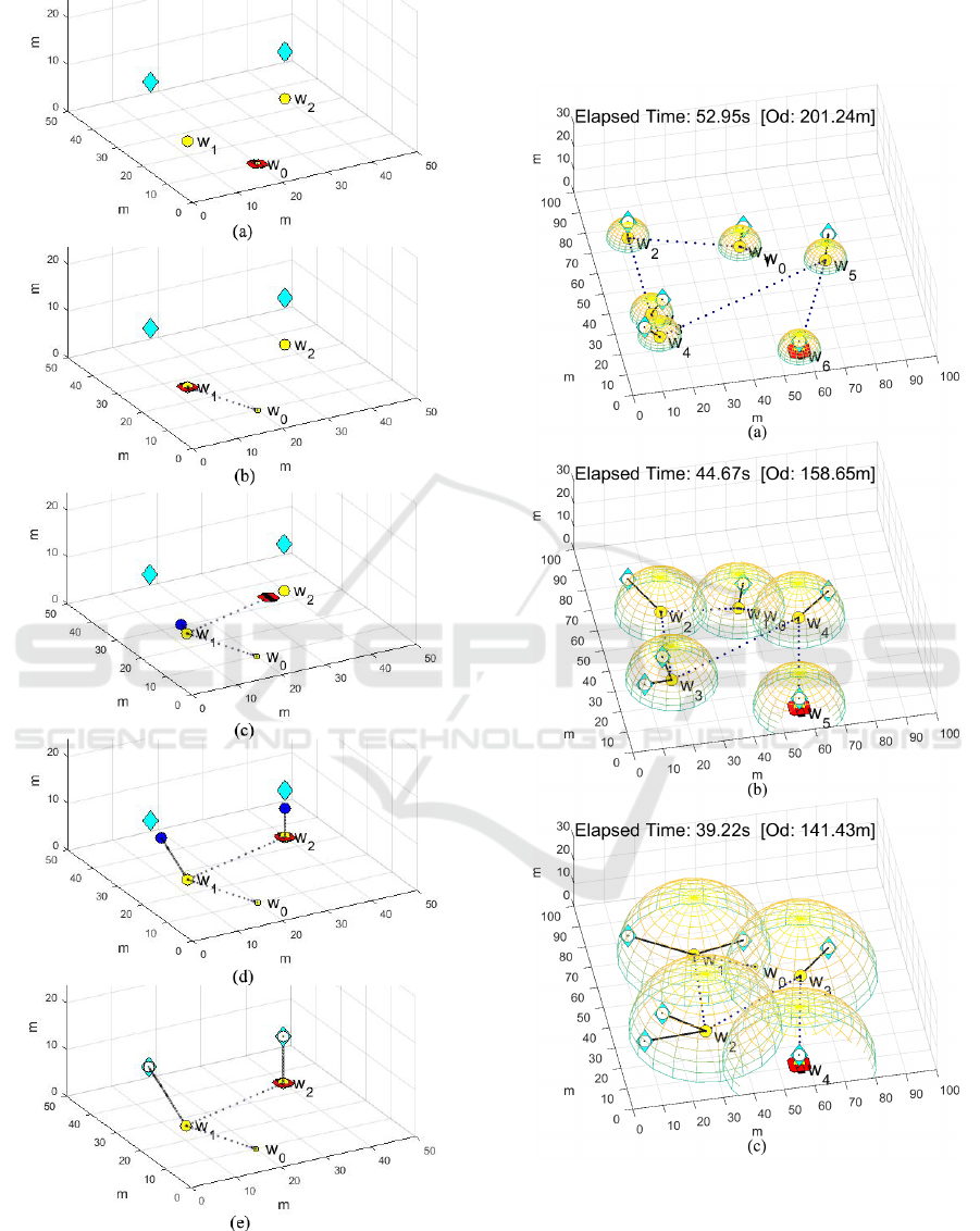
Figure 6: Deployment procedure. (a) Initial state (b) The
CR approaches to w
1
(c) The CR approaches to w
2
, and
first UAV moves to first task location (d) Two UAVs are
approaching (e) All UAVs reach their assigned locations.
Figure 7: Deployment Example for six tasks in (100m ×
100m×30m). We set v
max
C
= 15.0m/s,w
C
= 3.0rad/s,a
C
=
10.0m/s
2
,τ = 4.0s, and v
R
= 1.0m/s. (a) d
max
= 7.0m (b)
d
max
= 15.0m (c) d
max
= 25.0m (d) d
max
= 35.0m.
Efficient Deployment of Energy-constrained Unmanned Aerial Vehicles in 3-dimensional Space
451
