Calculation of the Boundaries and Barriers of the Workspace of a

Redundant Serial-parallel Robot using the Inverse Kinematics

Adri´an Peidr´o,

Oscar Reinoso, Arturo Gil, Jos´e Mar´ıa Mar´ın, Luis Pay´a and Yerai Berenguer

Systems Engineering and Automation Department, Miguel Hern´andez University, 03202, Elche, Spain

Keywords:

Robot Manipulator, Redundant Robot, Workspace, Inverse Kinematics, Discretization Methods.

Abstract:

This paper presents the workspace analysis of a redundant serial-parallel robot. Due to the complexity of the

robot, the complex constraints (joint limits and no-interference between the legs of the robot), and the globally

serial structure of the robot, a discretization method based on the forward kinematics would be most appro-

priate to compute the workspace. However, this widely used method can only obtain the external boundaries

of the workspace, missing the internal barriers that hinder the motion of the robot, which may exist inside the

boundaries. To avoid missing these barriers, we use a discretization method that uses the solution of the inverse

kinematic problem of the robot. By studying the feasibility of attaining a desired position and orientation by

the different branches of the solution to the inverse kinematics, the proposed discretization method is able to

obtain both the external boundaries and the internal barriers of the workspace. Some examples are presented

to show the importance of these internal barriers in the motions of the robot inside the workspace.

1 INTRODUCTION

The workspace of a robot manipulator, which is the

set of positions and orientations that its end-effector

can reach, is very important for designing the robot

and planning its movements. There are many meth-

ods to calculate the workspace of robots, but most of

them can be classiﬁed into three main groups (Merlet,

2006): geometrical methods, singularity-based meth-

ods and discretization methods.

The geometrical methods are especially useful for

parallel robots, in which the end-effector is controlled

by two or more kinematic chains actuating in paral-

lel. These methods obtain ﬁrst the workspace asso-

ciated with each kinematic chain individually. Such

individual workspaces usually are simple geometrical

objects, such as annuli (Merlet et al., 1998), spher-

ical shells (Gosselin, 1990) or tori (Liu and Wang,

2014). After obtaining the individual workspaces, the

workspace of the complete robot is obtained as the

intersection of these individual workspaces. These

methods are very fast and efﬁcient, but they are

also limited since they are only available for speciﬁc

robots. Moreover, with these methods it may be very

difﬁcult to take into account some restrictions in the

calculation of the workspace, such as the existence of

joint limits, or the condition that mechanical interfer-

ences between different bodies should not occur.

The singularity-based methods begin by writing

all the kinematic restrictions of the robot (including

joint limits) as a system of equations. Next, the Ja-

cobian matrix of this system with respect to all the

involved variables is derived, excluding the variables

that deﬁne the position and orientation of the end-

effector. Then, the boundaries of the workspace can

be obtained as the set of conﬁgurations of the robot

for which the mentioned Jacobian matrix is not full-

rank. These conﬁgurations that produce the rank de-

ﬁciency of the Jacobian matrix may be found analyti-

cally (Abdel-Malek and Yang, 2006; Abdel-Malek et

al., 2000) or numerically (Haug et al., 1996; Bohigas

et al., 2012). The main problem of the singularity-

based methods is the fact that all the constraints must

be written as equalities, which may result in too large

systems of equations. Moreover, some restrictions

cannot be modeled as equality constraints, like the

condition of no-interference between different bodies.

Finally, the discretization methods are very ﬂexi-

ble and can easily deal with all types of constraints, al-

though they can be very computer-intensive. The dis-

cretization methods consist of discretizing the Carte-

sian (or joint) space into a regular or randomized grid

of nodes, and solving the inverse (or forward) kine-

matic problem of the robot for each node to obtain

the complete conﬁguration of the robot (Macho et

al., 2009; Bonev and Ryu, 2001; Pisla et al., 2013;

412

Peidró, A., Reinoso, Ó., Gil, A., Marín, J., Payá, L. and Berenguer, Y.

Calculation of the Boundaries and Barriers of the Workspace of a Redundant Serial-parallel Robot using the Inverse Kinematics.

DOI: 10.5220/0005984704120420

In Proceedings of the 13th International Conference on Informatics in Control, Automation and Robotics (ICINCO 2016) - Volume 2, pages 412-420

ISBN: 978-989-758-198-4

Cervantes-S´anchez et al., 2000). Then, it is checked if

the obtained conﬁguration satisﬁes all the considered

constraints (e.g. joint limits or no-interference), in

which case the conﬁguration is stored as a workspace

point. Since the forward kinematic problem is usually

easier to solve in serial robots than the inverse prob-

lem, it is more convenient to discretize the joint space

for these robots. On the contrary, the inverse kine-

matic problem is usually simpler for parallel robots

than the forward problem, therefore the Cartesian

space is usually discretized for them.

This paper presents the calculation of the

workspace of a redundant serial-parallel robot with

ten degrees of freedom, using a discretization method

and the solution of the inverse kinematic problem.

The robot is composed of some parallel mechanisms

connected in series, which grants it a globally se-

rial architecture. Both its globally serial structure

and its kinematic redundancy make its forward kine-

matic problem much simpler than its inverse kine-

matic problem. Thus, a method based on discretiz-

ing its joint space and solving the forward kinemat-

ics would be more appropriate for calculating its

workspace. Nevertheless, this method misses impor-

tant information regarding the internal structure of the

workspace, which is crucial for planning the move-

ments of the robot. For example, Figure 1a shows the

workspace that is obtained when sampling the joint

space of the robot and solving its forward kinematic

problem. This method simply generates positions for

the end-effector and “populates” the workspace with

these positions. As a result, this method only yields

the external boundaries of the workspace. However,

a more careful analysis of the workspace, as the one

presented in this paper, reveals the existence of inter-

nal barriers inside the workspace, as shown in Figure

1b. These internal barriers, which cannot be detected

when generating the workspace by using the forward

kinematics, are very important for planning the move-

ments of the robot, since they imply motion impedi-

ments.

(a) (b)

Internal barriers

Figure 1: (a) Workspace generated by discretizing the joint

space and generating positions solving the forward kine-

matic problem. This method only yields the external bound-

aries. (b) Actually, the method based on the forward kine-

matics misses existing internal barriers that hinder the mo-

tion of the robot.

In this paper, we present a discretization method to

calculate the workspace of the aforementioned serial-

parallel robot, including the internal barriers that lie

inside the external boundaries. To this end, the Carte-

sian space is discretized instead of the joint space,

and the inverse kinematic problem is solved instead

of the forward kinematics. Although the robot is re-

dundant, the different branches of the solution to its

inverse kinematic problem can be exploited to obtain

the workspace boundaries and the internal barriers,

as this paper shows. After presenting the proposed

method, some examples are used to show the impor-

tance of the internal barriers of the workspace in the

planning of the movements of the robot.

The remainder of this paper is organized as fol-

lows. Section 2 presents a ten-degrees-of-freedom

serial-parallel robot and reviews the solution to the

inverse kinematic problem of this robot. Next, Sec-

tion 3 presents a method based on the solution of

the inverse kinematics to compute the workspace of

the robot, including the barriers present inside the

workspace. Section 4 presents some examples of the

application of the proposed method to calculate dif-

ferent workspaces, and analyzes the effects of the in-

ternal barriers on the motion of the robot. Finally,

Section 5 concludes this paper.

2 INVERSE KINEMATICS OF A

SERIAL-PARALLEL ROBOT

This section reviews the solution of the inverse kine-

matic problem of the redundant serial-parallel robot

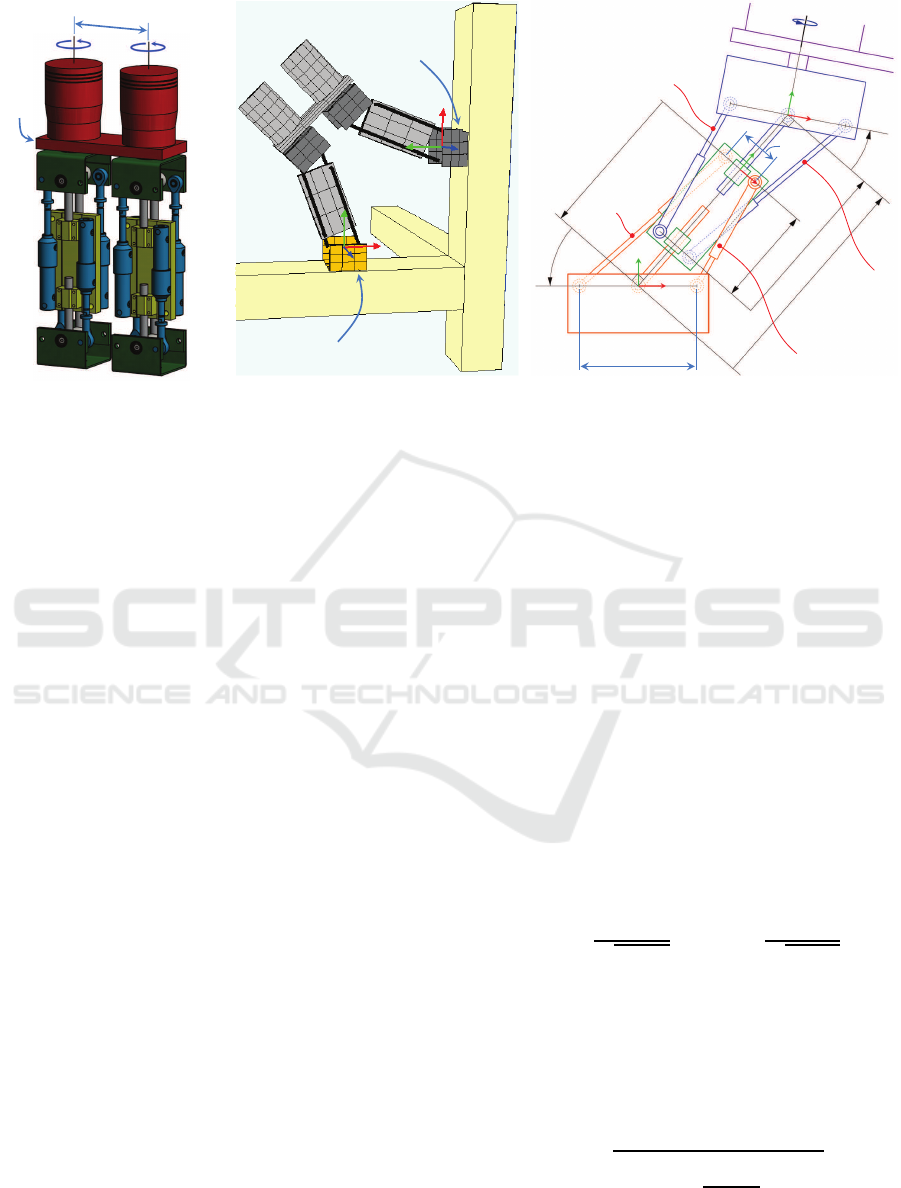
shown in Figure 2a. This robot is designed to climb

and explore 3D structures, like metallic bridges, to

inspect and maintain them. Its feet carry magnets to

adhere to the climbed structure. Figure 2b shows an

example of the robot performing a transition between

two perpendicular beams of a 3D structure.

The robot is biped, and each leg j ∈ {A, B} is

composed of two parallel mechanisms connected in

series. In each leg j, the i-th parallel mechanism

(i ∈ {1, 2}) has two linear actuators with lengths u

and v

(see Figure 2c). Furthermore, each leg is con-

nected to the hip H through one revolute actuated

joint, which rotates the leg an angle θ

with respect

to the hip. Thus, the robot has ten degrees of free-

dom. The joint coordinates associated to these ten

degrees of freedom are the lengths of the eight linear

actuators and the two rotated angles of the hip, i.e.

q = [u

, v

, u

, v

, u

, v

, u

, v

, θ

]

The geometric design of the robot depends on

four parameters, which can be seen in Figure 2: the

width b and length h of the central body of the legs,

Calculation of the Boundaries and Barriers of the Workspace of a Redundant Serial-parallel Robot using the Inverse Kinematics

413

Hip H

Leg A

Leg B

Foot A Foot B

(a) (b)

(c)

Foot j

Hip H

Foot A

Foot B

Figure 2: (a) CAD model of the serial-parallel robot studied in this paper. (b) Example of the robot performing a transition

between two perpendicular beams in a 3D structure. (c) Detailed view of the kinematics of the leg j of the robot (j ∈ {A, B}).

the width p of the feet, and the separation t between

the rotations of the hip. Furthermore, in practice the

lengths of the linear actuators should be limited, i.e.

, v

∈ [ρ

, ρ

+ ∆ρ], where ρ

> 0 is the minimum

length of these actuators and ∆ρ > 0 is their stroke.

Thus, the parameters ρ

and ∆ρ will also be regarded

as design parameters of the robot.

The inverse kinematic problem of this robot was

solved in (Peidro et al., 2015), and the solution will be

summarized here since we will use it to compute the

workspace of the studied robot. The inverse kinematic

problem consists of ﬁnding the values of the joint co-

ordinates q necessary to attain a desired position and

orientation for the foot B relative to the foot A, given

by the following homogeneous transform matrix T







0 0 0 1







(1)

where r

are the components of the rotation matrix

that deﬁnes the orientation of the foot B with respect

to the foot A and p = [p

, p

]

is the position vec-

tor of the foot B relative to the foot A.

As stated above, the inverse kinematic problem

consists of calculating the vector q of the joint co-

ordinates from the relative position and orientation

between the feet of the robot, given by the matrix

. However, as demonstrated in (Peidro et al.,

2015), the inverse kinematic problem becomes eas-

ier by deﬁning a set of intermediate joint coordi-

nates

q = [ϕ

, ϕ

, y

, θ

]

which can be solved more easily in terms of T

(the

geometrical meaning of each intermediate joint coor-

dinate is shown in Figure 2c). Then, it can be shown

that after solving

q, the intermediate joint coordi-

nates unequivocally determine the joint coordinates

q. The solution for the intermediate joint coordinates

depends on the desired orientation, distinguishing two

cases (Peidro et al., 2015).

2.1 Case 1: r

6= 1

Assume that the four intermediate joint coordinates

{ϕ

, y

} are known. In that case, it can be

shown that the remaining six intermediate joint coor-

dinates {ϕ

, ϕ

, y

, θ

} can be calculated in

terms of {ϕ

, y

} by performing the following oper-

ations. First, ϕ

is calculated as follows:

= σ

1− r

, c

= σ

−r

1− r

(2)

= ϕ

− atan2(s

, c

) (3)

where σ

∈ {−1, 1} and atan2(sin(ψ), cos(ψ)) is the

inverse tangent function that uses the sine and the co-

sine of an angle ψ to calculate the angle in the correct

quadrant. Next, θ

is calculated as follows:

= −

+ r

+ p

(4)

= σ

1− s

(5)

= atan2(s

, c

) (6)

ICINCO 2016 - 13th International Conference on Informatics in Control, Automation and Robotics

414

where σ

∈ {−1, 1}, s

= sin(ϕ

), and c

cos(ϕ

). Following, θ

can be calculated as:

= r

+ c

− s

) (7)

= r

− s

) (8)

= atan2(s

, c

) (9)

Finally, the remaining intermediate joint coordinates

{ϕ

, ϕ

, y

} can be calculated as follows:

= s

+ c

, c

= s

+ c

(10)

Ω

= r

+ r

+ p

− tc

(11)

Ω

= r

+ r

+ p

+ tc

(12)

Ω

+ Ω

(13)

= atan2(Ω

, Ω

) (14)

= ϕ

− atan2(s

, c

) (15)

2.2 Case 2: r

= 1

In this case, we assume that the values of the ﬁve

intermediate joint coordinates {ϕ

, ϕ

, y

}

are known. Then, by deﬁning s

= sin(ϕ

−ϕ

) and

= cos(ϕ

− ϕ

), we can still compute the values

of the remaining ﬁve intermediate joint coordinates

{ϕ

, ϕ

, y

, θ

} using Eqs. (4) to (15).

2.3 Feasible Regions

The solutions described in subsections 2.1 and 2.2 as-

sume that some of the intermediate joint coordinates

are known, and compute the remaining intermediate

joint coordinates in terms of the former. This is due

to the kinematic redundancy of the robot: ﬁxing the

position and orientation of one foot with respect to

the other foot only provides six independent equations

(three for the position and three for the orientation)

to calculate ten unknown intermediate joint coordi-

nates. Thus, six independent equations only allow us

to calculate six intermediate joint coordinates in terms

of the remaining four, as described in subsection 2.1.

Moreover, when the desired orientation between the

feet satisﬁes r

= 1, ϕ

cannot be determined from

the equations and its value must also be assumed to

be known (subsection 2.2).

According to the solutions described in the pre-

vious subsections, the solution of the inverse kine-

matic problem for a given desired position and orien-

tation is a four-dimensional set in the ten-dimensional

space of the intermediate joint coordinates (or a ﬁve-

dimensional set if the desired orientation satisﬁes

= 1). This is because the ten intermediate joint

coordinates have been solved in terms of four (or

ﬁve) of the intermediate joint coordinates [called de-

cision variables in (Peidro et al., 2015)], whose values

can be freely decided. In contrast, in non-redundant

robots the solution to the inverse kinematics is a set

of isolated points in the joint space (i.e., a zero-

dimensional set). Due to the high dimensionality of

the solution sets in this robot, it is not possible to

represent graphically the complete solutions to the in-

verse kinematics.

However, as demonstrated in (Peidro et al., 2015),

it is possible to reduce the dimensionality of these

solution sets without losing relevant information, ob-

taining an alternative and more compact representa-

tion of the solutions of the inverse kinematic problem.

This reduction of dimensionality is based on the fact

that not all the decision variables (i.e. the four or ﬁve

intermediate joint coordinates in terms of which the

remaining unknowns are calculated) are equally im-

portant to determine the posture of the robot. In fact,

it can be shown that after ﬁxing the values of the de-

cision variables {ϕ

, y

} (and also ϕ

, if r

= 1),

the overall posture of the robot is determined, and

the remaining decision variables {y

, y

} only pro-

duce small internal motions of the central bodies of

the legs along the legs, which do not affect the over-

all posture of the robot. Since the overall posture of

the robot only depends on {ϕ

, y

} (and also ϕ

, if

= 1), we can focus only on these two (or three)

variables to analyze the solutions of the inverse kine-

matic problem, and use this information to discard the

pairs {ϕ

, y

} that yield a forbidden posture in which

the legs of the robot interfere, for example.

Exploiting the previous idea regarding the possi-

bility of reducing the dimension of the solution sets,

(Peidro et al., 2015) developed a Monte Carlo algo-

rithm to obtain the regions R

of the ϕ

-y

plane

(or the regions of the ϕ

-ϕ

-y

space, if r

= 1)

which allow the robot to attain a desired position and

orientation T

satisfying the joint limits, and they

called these regions feasible regions. Any point of

these feasible regions yields a valid solution of the

inverse kinematic problem, satisfying the condition

that the lengths of the eight linear actuators of the

robot should be between the joint limits [ρ

, ρ

+ ∆ρ].

In this paper, we will impose an additional condi-

tion to calculate the feasible regions: in order for a

pair {ϕ

, y

} (or triplet {ϕ

, ϕ

, y

}, if r

= 1)

to belong to the feasible regions R

, the posture cor-

responding to that pair (or triplet) should not pro-

duce mechanical interferences between the legs of the

robot. To check this condition of no-interference be-

tween the legs, the Separating Axis Theorem will be

used (Ericson, 2004). This will be explained in Sec-

tion 4 in more detail.

Calculation of the Boundaries and Barriers of the Workspace of a Redundant Serial-parallel Robot using the Inverse Kinematics

415

According to subsection 2.1, the solution to the

inverse kinematics depends on two binary variables

, σ

∈ { −1, 1} when the desired orientation satis-

ﬁes r

6= 1. Each combination of these binary vari-

ables will yield a different feasible region R

, which

corresponds to a different branch of the solution to

the inverse kinematics. Thus, when r

6= 1, the so-

lution to the inverse kinematics will have four dif-

ferent branches, identiﬁed by the four possible com-

binations (σ

, σ

) of these binary variables: (1, 1),

(1, −1), (−1, 1), (−1, −1). If the desired orienta-

tion satisﬁes r

= 1, then according to subsection 2.2

only the binary variable σ

is involved in the solu-

tion of the inverse kinematics. Thus, the inverse kine-

matic problem will only have two different branches

in that case, one branch corresponding to σ

= 1 and

the other branch corresponding to σ

= −1.

3 OBTAINING THE WORKSPACE

USING THE INVERSE

KINEMATICS

In this section, we will describe how the solution to

the inverse kinematic problem, described in Section

2, can be used to obtain the workspace of the serial-

parallel robot studied in this paper, including its ex-

ternal boundaries and internal barriers.

According to the previous section, the solution to

the inverse kinematic problem of the serial-parallel

robot studied in this paper can be summarized as fol-

lows. Given a desired position and orientation be-

tween the feet of the robot, encoded by the homoge-

neous transformation matrix T

deﬁned in Eq. (1),

the solution to the inverse kinematics depends on r

• If the desired orientation satisﬁes r

6= 1, then the

solution to the inverse kinematics can be repre-

sented by a feasible region R

in the ϕ

-y

plane,

such that any point of this region corresponds to a

posture that allows the robot to attain the desired

position and orientation T

satisfying the joint

limits of the linear actuators and guaranteeing that

the legs of the robot do not interfere. Moreover,

there exist four different branches for the solution,

i.e. four different feasible regions R

correspond-

ing to the four possible combinations of the binary

variables σ

and σ

• If the desired orientation satisﬁes r

= 1, the so-

lution to the inverse kinematics can be represented

by a feasible region R

in the ϕ

-ϕ

-y

space,

such that any point of R

yields a posture that al-

lows the robot to attain the desired position and

orientation T

satisfying the joint limits of the

linear actuators and guaranteeing that the legs of

the robot do not interfere. In this case, there exist

two different branches for the solution, i.e. two

different feasible regions R

, one region per each

value of the binary variable σ

Once the solution to the inverse kinematics is

available (including all the branches of this solution),

the workspace boundaries and barriers can be ob-

tained using a discretization algorithm explained next.

The workspace of this robot can be deﬁned as the

set of positions and orientations that the foot B can at-

tain with respect to the foot A. Such a workspace is a

six-dimensional set, since the position and orientation

of the foot B relative to the foot A can be represented

by three translations p = [p

, p

]

and three rota-

tions r = [α, β, γ]

(where α, β and γ are Euler angles).

To calculate the workspace, the six-dimensional space

of the variables {p

, p

, α, β, γ} is discretized into a

regular grid of nodes. For example, we may approx-

imate each axis of this six-dimensional space by n

nodes regularly distributed between two limits, which

yields an overall grid of n

nodes. Then, for each node

of this grid, the inverse kinematic problem if solved to

check if the node is attainable by each branch of the

solution of the inverse kinematics.

For each branch i of the solution to the inverse

kinematics, we create a list WS

of the nodes that

can be reached using that branch. After the algorithm

has checked all the nodes of the grid, the list WS

an approximation of the workspace associated to the

branch i, since it contains all the positions and orien-

tations that can be reached with that branch. Then,

the boundaries of the workspace associated to the i-th

branch can be approximated by the nodes contained in

which have at least one unreachable neighboring

node (i.e., a neighboring node not contained in WS

After obtaining the boundaries of the workspaces as-

sociated to the different branches, the boundaries of

all the branches can be joined to obtain the bound-

aries and barriers of the complete workspace.

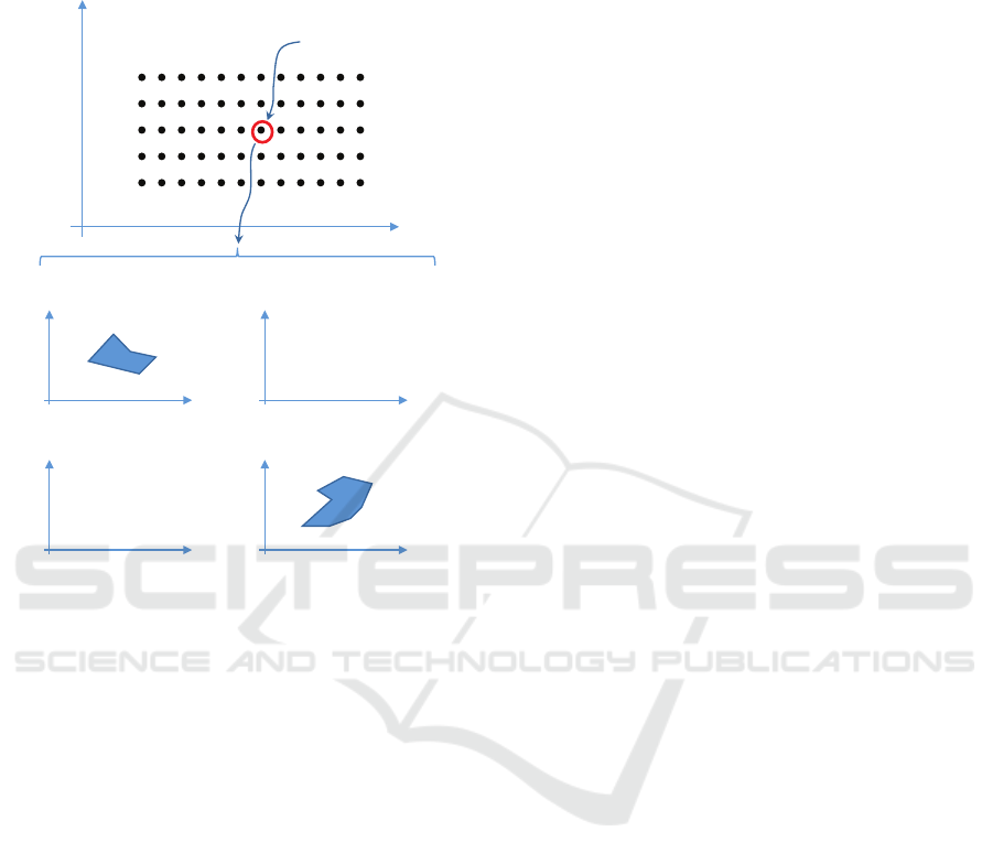
To determine if an arbitrary node of the grid is at-

tainable using a given branch i of the inverse kinemat-

ics, the feasible region R

associated to that branch is

calculated using the Monte Carlo algorithm described

in (Peidro et al., 2015). If the region R

is empty, then

it is considered that the node is not attainable by the i-

th branch, and the node is not included in the list WS

(see Figure 3). The mentioned Monte Carlo algorithm

generates the region R

by randomly sampling points

in the ϕ

-y

plane (or in the ϕ

-ϕ

-y

space, if

= 1). If the posture generated by each randomly

sampled point satisﬁes the joint limits of the linear ac-

tuators, and if the legs do not interfere, then that point

is stored as a point of the feasible region R

. In this

ICINCO 2016 - 13th International Conference on Informatics in Control, Automation and Robotics

416

way, a discrete approximation of the region R

can be

obtained by sampling a large number of points in the

-y

plane (or in the ϕ

-ϕ

-y

space).

Node k

Branchı

ı

= 1

Branchı

ı

= -1

Branchı

= -ı

= 1

Branchı

= -ı

= -1

Figure 3: A 2D example that illustrates the process to deter-

mine whether a given node k of the potential workspace is

reachable or not. For a given node k, the feasible regions R

are calculated using all the branches of the solution of the

inverse kinematic problem. In this case, the node k belongs

only to the workspaces of the branches (1, 1) and (−1, −1)

since these are the only branches leading to non-empty fea-

sible regions R

Note that it is sufﬁcient to ﬁnd a single point be-

longing to R

to guarantee that R

is not empty and

classify the corresponding node of the workspace as

attainable. However, checking if R

is empty (and

classifying the corresponding node as unattainable by

the i-th branch of the inverse kinematics) is not that

easy, since one would need to explore exhaustively

the ϕ

-y

plane (or the ϕ

-ϕ

-y

space) to guaran-

tee that this plane (space) does not have points satis-

fying all the constraints (i.e., to guarantee that R

empty). Since it is not feasible to perform such an

exhaustive search to check if R

is empty, this prob-

lem is practically solved by establishing a maximum

number n

of attempts to generate a point in R

. Then,

the aforementioned Monte Carlo algorithm begins to

randomly sample points in the ϕ

-y

plane (or in

the ϕ

-ϕ

-y

space, if r

= 1). If it ﬁnds a point

that satisﬁes all the constraints (joint limits and no-

interference), the Monte Carlo algorithm stops: the

region R

is not empty (it contains at least one point)

and the node is classiﬁed as attainable. If, on the con-

trary, the Monte Carlo algorithm has sampled n

ran-

dom points and none of them satisﬁes the constraints,

it is considered that R

is empty, which means that the

corresponding node cannot be attained by the consid-

ered branch of the inverse kinematics. Obviously, this

method will be more accurate when n

increases, but

the computation will also take more time, so a com-

promise between precision and computational cost is

necessary.

It should be remarked that the method described

in this section to compute the workspace is very

computer-intensive if we try to discretize and com-

pute the six-dimensional workspace of the variables

, p

, α, β, γ}, since the number of nodes to

check is n

(and, for each node, the feasible regions

must be obtained for the different branches of

the inverse kinematics). Moreover, a six-dimensional

workspace cannot be represented graphically. For

these reasons, and to decrease the computational

cost, we will ﬁx some of these six variables to ob-

tain lower-dimensional workspaces that can be repre-

sented graphically and are more easy to understand,

such as the constant-orientation workspace (i.e., the

set of positions that can be attained by the foot B with

respect to the foot A when the relative orientation be-

tween the feet is constant). The constant-orientation

workspace is very useful when planning some move-

ments which are necessary to explore a 3D structure,

such as when performing a transition between dif-

ferent beams (see Figure 2b). In the following sec-

tion, we will illustrate the algorithm described in the

present section using some examples.

4 EXAMPLES

This section presents some examples of the applica-

tion of the method described in Section 3 to compute

different workspaces of the studied robot. For the

next examples, the geometric design parameters of the

robot are: b = p = 4, h = 16, t = 15.6, ρ

= 19, and

∆ρ = 7.5 (all in cm). In all the examples of this sec-

tion, we will discretize the workspace into n

= 200

points in each axis. Moreover, we will sample a max-

imum of n

= 5000 random points before deciding

that the feasible region R

(of valid postures that yield

a given position and orientation between the feet) is

empty (n

was deﬁned in Section 3). In all the exam-

ples, we will assume that the foot A is ﬁrmly attached

to the structure, and we will compute the set of posi-

tions that the foot B (which is free to move) can reach.

Calculation of the Boundaries and Barriers of the Workspace of a Redundant Serial-parallel Robot using the Inverse Kinematics

417

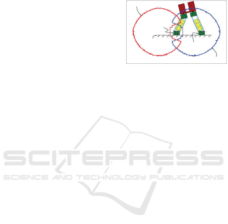
4.1 Example 1

In this example, we are interested in obtaining a

constant-orientation workspace, i.e. the set of attain-

able points by the foot B when the relative orienta-

tion between the feet is constant. More speciﬁcally,

we will study the workspace obtained when both feet

have the same orientation, which means that the ro-

tation submatrix of T

is the identity matrix. Fur-

thermore, we will be interested only in the intersec-

tion of such constant-orientation workspace with the

plane p

= 0, to study the planar motions of the robot

inside this constant-orientation workspace. Note that

the robot needs to perform motions of this type to

travel along a beam of a structure, as shown in Fig-

ure 4. The desired position and orientation will have

the following form for this example:







1 0 0 p

0 1 0 p

0 0 1 0

0 0 0 1







(16)

To apply the algorithm described in the previous

section, we will deﬁne a box B that encloses the

workspace in the p

-p

plane, and we will discretize

this box into a grid of 40000 nodes regularly dis-

tributed (200 nodes per each axis). Then, for each

node, we will solve the inverse kinematic problem us-

ing the matrix of Eq. (16) as the input, to check if each

node is attainable by the different branches of the in-

verse kinematics. The chosen box for this example

is B = {(p

, p

) : −80 cm ≤ p

≤ 80 cm, −50 cm ≤

≤ 50 cm}. Running the algorithm described in the

previous section for these parameters, the workspace

shown in Figure 4 is obtained. Note that, since in

this case r

= 1, according to Section 2.3 the solution

to the inverse kinematic problem in this case has two

branches: one for σ

= 1 and other for σ

= −1. The

workspaces associated to these branches are shown in

Figure 4 with different colors.

Note that this workspace is split into the compo-

nents associated with the two branches of the solu-

tion to the inverse kinematic problem. The complete

workspace (i.e. the union of the two components)

has a void around the foot A, which is necessary to

avoid the interferences between the legs. Accord-

ing to Figure 4, the robot cannot move the foot B

from one side of the workspace (e.g. the right half

the workspace, associated with the branch σ

= 1) to

the other side (e.g. the left half, associated with the

branch σ

= −1) keeping constant the orientation be-

tween the feet, since the workspaces associated with

both branches have boundaries in the middle of the

workspace, both above and below the foot A. This is

-80

-50

Beam

Branch ı

= -1

Branch ı

= 1

Foot A

Foot B

Figure 4: Planar constant-orientation workspace that pro-

vides the points at which the foot B can be placed with the

same orientation as the foot A. This constant-orientation

workspace is useful to plan movements along the direction

of the beam. The workspaces associated with the branches

= −1 and σ

= 1 are represented in red and blue colors,

respectively.

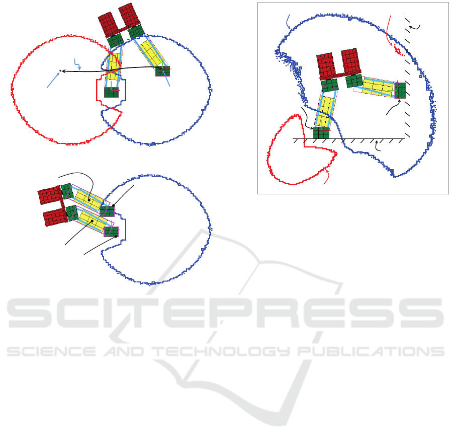
illustrated in Figure 5, where the robot starts at an ini-

tial point in the workspace associated with the branch

= 1, and tries to describe a trajectory towards the

left half of the workspace (see Figure 5a). However,

the trajectory cannot be completed because the robot

cannot cross the boundaries of the component of the

workspace in which it moves. This boundary is orig-

inated from the fact that the legs cannot interfere: as

Figure 5b shows, when the foot B is close to the men-

tioned boundary, both legs are about to intersect.

To check if the two legs interfere in all the ex-

amples of this paper, the Separating Axis Theorem is

used (Ericson, 2004). Each leg can be approximated

by the union of two cuboids (also known as rectan-

gular parallelepipeds): one cuboid encloses the foot,

and the other cuboid encloses the central body of the

leg, including the linear actuators (these cuboids are

represented in magenta in Figure 5b). Then, the two

legs will interfere if one of the cuboids of one leg in-

tersects one of the cuboids of the other leg. Since the

cuboids are convex shapes, the Separating Axis The-

orem can easily be used to check if they intersect.

4.2 Example 2

In this example, the objective is to ﬁnd the planar

constant-orientation workspace deﬁned by the follow-

ing homogeneous transformation matrix between the

feet of the robot:







0 −1 0 p

1 0 0 p

0 0 1 0

0 0 0 1







(17)

This orientation is a rotation of 90

◦

about the Z axis,

which is necessary to perform a transition between

ICINCO 2016 - 13th International Conference on Informatics in Control, Automation and Robotics

418

(a)

(b)

Initial position

Final position

Trajectory

Foot A

Foot B

Central body

of the leg A

Central body of

the leg B

Figure 5: (a) A trajectory between both components of the

workspace. (b) The robot cannot reach the left component

because it cannot cross a boundary of the component in

which it moves (the right component). When approaching

the boundary, the legs are about to intersect: the foot B is

almost touching the central body of the leg A. To cross the

boundary, an interference between these two bodies would

be necessary.

two perpendicular beams in a structure, as shown in

Figures 2b and 6. Again, we are interested only in the

intersection of this constant-orientation workspace

with the plane p

= 0, since the motion necessary to

perform such a transition is planar.

Next, the algorithm described in Section 3 is ap-

plied, discretizing the following box B into a grid of

40000 nodes (200 nodes per axis): B = {(p

, p

) :

−40 cm ≤ p

≤ 80 cm, −40 cm ≤ p

≤ 80 cm}. The

resulting workspace is shown in Figure 6. Again,

since the desired orientation satisﬁes r

= 1, the

solution to the inverse kinematic problem has two

branches, one for σ

= 1 (shown in blue in Figure 6)

and other for σ

= −1 (shown in red in Figure 6).

In this case, the workspace attainable using the

branch σ

= −1 of the solution to the inverse kine-

matic problem is smaller than the workspace associ-

ated with the branch σ

= 1. Note that the workspace

associated with the branch σ

= −1 has two compo-

nents: a big one, which is close to the foot A in Figure

-40

Foot A

Foot B

Beam 1

Beam 2

Branch ı

= -1

Branch ı

= 1

Branch ı

= -1

Figure 6: Planar constant-orientation workspace containing

all the points of the plane p

= 0 that can be reached with

the foot B rotated 90

◦

about the Z axis with respect to the

foot A.

6, and a smaller one, which is close to the beam 2 in

the same ﬁgure. Actually, the shape of the smaller

component cannot be appreciated very well in Fig-

ure 6. However, a more precise approximation of that

component can be obtained if the algorithm described

in Section 3 is executed again discretizing a smaller

box B that encloses only the area around the men-

tioned small component of the workspace, instead of

using a big box that contains all the components as

shown in Figure 6.

The posture of the robot shown in Figure 6, with

the foot B placed on the beam 2, is obtained using the

branch σ

= 1 of the solution to the inverse kinemat-

ics. However, according to the same ﬁgure, it would

be also possible to place the foot B on the beam 2

using the branch σ

= −1, since this branch yields

a small component of the workspace near the beam

2 (i.e., the small component described in the previ-

ous paragraph). This is checked in Figure 7, which

shows a posture of the robot that places the foot B at

a point of the smallest of the two workspace compo-

nents associated with the branch σ

= −1. As this ﬁg-

ure shows, using the branch σ

= −1, the foot B can

also be effectively placed on the beam 2 with the de-

sired orientation. However, in this posture, the hip of

the robot intersects the beams, so this would not be a

feasible solution in practice. This unfeasibility can be

easily detected by the presented method if we include

the condition that no part of the robot should intersect

the obstacles of the environment, using a similar pro-

cedure to the method used to check if different legs

intersect, described in subsection 4.1.

Calculation of the Boundaries and Barriers of the Workspace of a Redundant Serial-parallel Robot using the Inverse Kinematics

419

Collisions with the

beams of the structure

Beam 2

Beam 1

Figure 7: A posture which places the foot B on the beam 2

with the desired orientation, using the branch σ

= −1. In

this posture, the robot collides with the structure.

5 CONCLUSIONS

This paper has presented a discretization method to

calculate the workspace of a serial-parallel redundant

robot using the solution to its inverse kinematic prob-

lem. In contrast to the methods based on the for-

ward kinematics, the proposed method is able to ob-

tain both the external boundaries and the internal bar-

riers of the workspace. Using this method, we have

analyzed the negative effects of the internal barriers

on the movements of the robot inside its workspace.

In the future, we will solve the path planning prob-

lem of this robot. We hope that the analysis presented

in this paper will be very useful to plan the move-

ments of the robot, since the presented method gener-

ates workspace maps that allow the robot to navigate

safely through its workspace, knowing the positions

at which the actuators attain the joint limits, or the

positions where the legs of the robot would collide.

ACKNOWLEDGEMENTS

This work has been supported by the Spanish Min-

istry of Education through grant FPU13/00413, by

the Spanish Ministry of Economy through project

DPI2013-41557-P, and by the Generalitat Valenciana

through project AICO/2015/021.

REFERENCES

Abdel-Malek, K., and Yang, J. (2006). Workspace bound-

aries of serial manipulators using manifold stratiﬁca-

tion. The International Journal of Advanced Manufac-

turing Technology, Vol. 28(11), pp. 1211–1229.

Abdel-Malek, K., Yeh, H.J., and Othman, S.(2000). Interior

and exterior boundaries to the workspace of mechan-

ical manipulators. Robotics and Computer-Integrated

Manufacturing, Vol. 16(5), pp. 365–376.

Bohigas, O., Manubens, M., and Ros, L. (2012). A Com-

plete Method for Workspace Boundary Determination

on General Structure Manipulators. IEEE Transac-

tions on Robotics, Vol. 28(5), pp. 993–1006.

Bonev, I.A., and Ryu, J. (2001). A new approach to orienta-

tion workspace analysis of 6-DOF parallel manipula-

tors. Mechanism and Machine Theory, Vol. 36(1), pp.

15–28.

Cervantes-S´anchez, J.J., Hern´andez-Rodr´ıguez, J.C., and

Rend´on-S´anchez, J.G. (2000). On the workspace,

assembly conﬁgurations and singularity curves of

the RRRRR-type planar manipulator. Mechanism and

Machine Theory, Vol. 35(8), pp. 1117–1139.

Ericson, C. (2004). Real-Time Collision Detection. CRC

Press.

Gosselin, C. (1990). Determination of the Workspace of

6-DOF Parallel Manipulators. ASME Journal of Me-

chanical Design, Vol. 112(3), pp. 331–336.

Haug, E.J., Luh, C.M., Adkins, F.A., and Wang, J.Y. (1996).

Numerical Algorithms for Mapping Boundaries of

Manipulator Workspaces. ASME Journal of Mechani-

cal Design, Vol. 118(2), pp. 228–234.

Liu, X.J., and Wang, J. (2014). Parallel Kinematics. Type,

Kinematics, and Optimal Design. Springer-Verlag

Berlin Heidelberg.

Macho, E., Altuzarra, O., Amezua, E., and Hernandez, A.

(2009). Obtaining conﬁguration space and singularity

maps for parallel manipulators. Mechanism and Ma-

chine Theory, Vol. 44(11), pp. 2110–2125.

Merlet, J.P. (1995). Determination of the orientation

workspace of parallel manipulators. Journal of Intel-

ligent and Robotic Systems, Vol. 13(2), pp. 143–160.

Merlet, J.P. (2006). Parallel Robots. Springer Netherlands.

Merlet, J.P., Gosselin, C.M., and Mouly, N. (1998).

Workspaces of planar parallel manipulators. Mecha-

nism and Machine Theory, Vol. 33(1-2), pp. 7–20.

Peidro, A., Gil, A., Marin, J.M., and Reinoso, O. (2015). In-

verse kinematic analysis of a redundant hybrid climb-

ing robot. International Journal of Advanced Robotic

Systems, 12:163, pp. 1–16.

Pisla, D., Szilaghyi, A., Vaida, C., and Plitea, N. (2013).

Kinematics and workspace modeling of a new hybrid

robot used in minimally invasive surgery. Robotics

and Computer-Integrated Manufacturing, Vol. 29(2),

pp. 463–474.

ICINCO 2016 - 13th International Conference on Informatics in Control, Automation and Robotics

420