Peaks Emergence Conditions in Free Movement Trajectories

of Linear Stable Systems

Nina A. Vunder and Anatoly V. Ushakov

ITMO University, Saint-Petersburg, Russia

Keywords: Linear System, Free Movement, Peak, Eigenvectors, Condition Number.

Abstract: The paper considers a asymptotically stable linear system with real eigenvalues of state matrix. It was found

that a peak in free movement trajectories arises. Geometric interpretation of peaks emergence was presented

through eigenspace. Quantitative estimate of the peak was obtained by using the condition number of matrix

of eigenvectors.

1 INTRODUCTION

The problem statement is to determine the

eigenvectors influence on free movement of

asymptotically stable continuous linear MIMO

system with real spectrum. It will be shown that

specific disposition of eigenvectors allows to peaking

effect (peak) emergence. It means that the norm of

state vector growths up and exceeds the norm of

initial conditions during some time and then

converges to zero. Necessary conditions of peak

emergence are the goal of research of current article.

2 GEOMETRIC

INTERPRETATION OF PEAKS

IN FREE MOVEMENT

TRAJECTORIES THROUGH

EIGENSPACE

Consider the linear system that is described as

() () ( ) ()

txxtFxtx



(1)

where

() ()

txx ,0

are vectors of initial and current

states of the system respectively;

is the state

matrix with eigenvalues

,1;0 =<

≠

for

ji ≠

and eigenvectors

{

}

niF

iiii

,1;: ==

ξλξξ

;

() ()

nnn

RFRkxx

∈∈ ;,0

The solution ((Andreev, 1976), (Gantmaher, 2004),

(Moler at al., 2003)) of the system (1) is

)0()( xetx

(2)

The vector

()

can be decomposed into the sum of

eigenvectors



)0(

ξγ

. Taking into account

properties of matrix exponential the solution (2) can

be write as follows



etx

)(

ξγ

(3)

where

,1;1 ==

∗

is the Euclidean norm on

R .

Definition 1. The system (1) has the peak in the

case if there is a vector

() ()

10:0 =xx

such that for

some value

0>t

the solution of the system satisfies

the condition

()

1>tx

(in general case

()

ax =0

where

0>a

- const).

Let us formulate a statement and let us prove it by

using geometric representations.

Statement 1. Necessary conditions of peaks

emergence in free movement trajectories of the

system (1) are:

1. There is at least one pair of eigenvectors

(

)

such that the angle between them is greater

than

in the subspace spanned by those

eigenvectors;

Vunder, N. and Ushakov, A.

Peaks Emergence Conditions in Free Movement Trajectories of Linear Stable Systems.

DOI: 10.5220/0005984605350538

In Proceedings of the 13th International Conference on Informatics in Control, Automation and Robotics (ICINCO 2016) - Volume 1, pages 535-538

ISBN: 978-989-758-198-4

535

2. There are eigenvalues

associated with

eigenvectors

such that

λλ

>> .

Let us prove

of the statement 1 by geometric way.

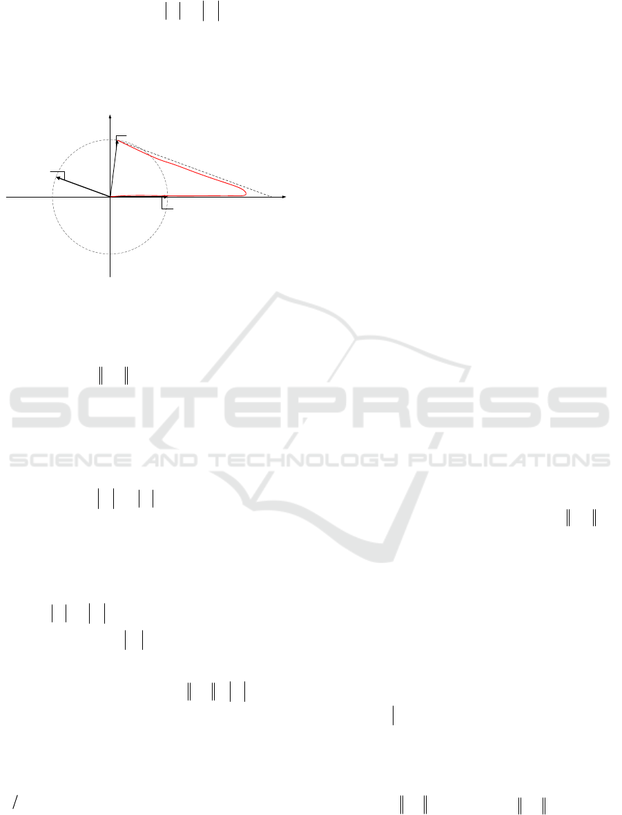
Let consider the linear span (subspace)

{

}

the vectors

(

)

which dispose at an obtuse angle

(see Fig. 1).

Figure 1.

Suppose the initial condition vector

()

of the

system (1) belongs to the span

()

{

}

,0 ∈

and

has the unit norm

()

10 =x

. Then the vector

()

can

be represented in the form

()

lljj

+=0

(4)

Now suppose the vector

()

is a bisector of the

angle between vectors

; then following relations

are true:

1,1, >>=

ljlj

γγγγ

Taking into account (3) we can write the

movement of system (1)

() ( )()

txxtx ,0=

in following

form

() ( )()

eetxxtx

γγ

+== ,0

(5)

If in (5)

λλ

>> and the system (1) is stable, then

from time

≈==

−

lПl

following conditions

become true:

() ( )()

etxxtxe

γγ

≅=≅ ,0;0

and

the norm of the vector

()

etx

≅ . The

statement 1 is proved.

Note 1.

It is obvious that there are no peaks in in

free movement trajectories of the system (1) if any of

following conditions holds:

1. The angle between vectors

is equal to

for any combinations of

2. The vector

()

is a bisector of the acute angle

between vectors

3. The vector

()

is inside the obtuse angle

between vectors

but not its bisector and one of

two following cases is realized:

{

}

0,1 →→

{

}

1,0 →→

for any combinations of eigenvalues

Let’s illustrate the validity of the statement 1 on

the example 1.

Example 1. Let the state matrix

of the system

(1) has eigenvectors

[] [ ]

ТТ

05.09987.0;01

−==

ξξ

such that they

have unit norm and condition 1 of statement 1 is

fulfilled. Let the state matrix

has the spectrum

{} ( )

[]

{}

50;1:0λarg

−=−==−==

FIdetF

such that the condition 2 of statement 1 is fulfilled.

Using the eigenspace and the spectrum, we have

[] []

500

726.9781

05.00

9987.01

500

05.00

9987.01













−













−













−













−













=Λ=

−

ξξ

MMF

where

- the matrix of eigenvectors.

Let the initial condition vector

()

[]

x 9997.00255.00 =

be a bisector of the angle

between

and has the unit norm

()

10 =x

Decompose the vector

()

into eigenvectors of the

matrix

()

994.199935.190

+=x

. Now, we

can write the free movement (5) of the system (1) with

the state matrix

in the following form

() ( )() ()()

.994.199935.19

0exp,0

eexFttxxtx

−−

=+===

λλ

γγ

It is obvious that the component

()

etx

994.19

−

of the free movement is close to zero at the time

()

0599.0ln

05.0

−

ελ

t . At the same time the

component

()

etx

−

9935.19

of the free

movement is equal to

()

0599.0

8311.189935.19

ξξ

−

etx

. Clearly, there is

a peak

()

max

of the norm

()

in the free

movement of the constructed two-dimensional

()

ICINCO 2016 - 13th International Conference on Informatics in Control, Automation and Robotics

536

system of type (1). The peak takes on the value

()

8324.17max =tx

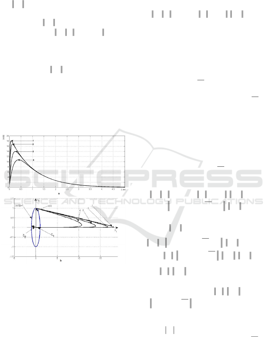
Let us confirm this result by observing the free

movement norm

()

. It is computed using the

following formula

() ()()

0exp xFttx =

. The

obtained curve is shown on Fig. 2.a (curve 1). The

curve confirms correctness of estimation of peak of

free movement trajectories obtained through the

geometrical interpretation. Fig.2.a and fig.2.b

demonstrate norms

()

of the system with same

eigenvectors but with following spectra:

{} { }

25;1

−=−==

(curve 2),

{} { }

10;1

−=−==

(curve 3),

{} { }

5;1

−=−==

(curve 4).

Moreover, fig. 2.a illustrates processes in norm,

and fig. 2.b does the same in phase space spanned by

eigenvectors.

Figure 2: Example of peaks.

3 ALGEBRAIC

INTERPRETATION.

CONDITION NUMBER AS А

QUANTITATIVE ESTIMATION

OF PEAKS

Consider the solution (2) of system (1) in order to

estimate the norm of possible peaks. If in (2) we turn

to norms ((Andreev, 1976), (Gantmaher, 2004),

(Moler at al., 2003), (Lancaster at al., 1985), (Golub

at al., 1976)), we get

() ()() () ()

0exp0exp xFtxFttx ⋅≤=

(6)

Recall that the system (1) satisfies conditions:

{}

()()

()













≠≠=

<=−=

jiJm

jii

при;0

;0;0detarg

λλλ

(7)

The matrix

can be represented in the form

1−

Λ=

(8)

where

{

}

nirowM

,1; ==

is matrix composed of

eigenvectors of matrix

such that the following

condition is true:

iii

;

{

}

nidiag

,1; ==Λ

diagonal matrix of eigenvalues. It is common

knowledge ((Gantmaher, 2004), (Lancaster at al.,

1985)) that the representation (8) holds for a matrix

function

(){}

of a matrix

()

() ()

1−

Λ= MMfFf

If the matrix function is the matrix exponential

() ( )

FtFf exp=

; then we can write

() ()

{}

.,1;

expexp

−

=Λ=

MnieMdiag

MMFt

(9)

Substituting (9) in (6), we get

() ()() () ()

{}

()

.0,1;

0exp0exp

xMnieMdiag

xFtxFttx

⋅==

=⋅≤=

−

(10)

Let us form inequality using (10) to obtain upper

estimate of

()

{}

()

{}

()

,0,1;

0,1;

xMniediagM

xMnieMdiagtx

⋅⋅=⋅≤

≤⋅=≤

−

(11)

where

1−

⋅ MM is equal to condition number

{}

((Golub, 1996), (Wilkinson, 1984, 1984),

(Zhang at al., 2014)):

{}

1−

⋅= MMMC

{}

eniediag

== ,1; , where

is maximum

eigenvalue of matrix

and it determines stability

index

(Andreev, 1976) of the system (1) in the

form

λη

. The condition number

{}

takes

minimal value if the matrix

{

}

nirowM

,1; ==

composed of vectors with unit norm. Then we can

write

Peaks Emergence Conditions in Free Movement Trajectories of Linear Stable Systems

537

() ()

{

}

()

xeMCtxrooftx

=≤

(12)

where

is modified matrix of eigenvectors of

matrix

such that it is composed of eigenvectors

with unit norm:

()

{

}

nidiagMM

,1;

=⋅=

−

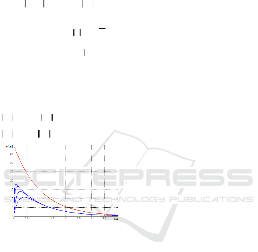
Example 2. Consider the system from example (1)

() () ( ) ()

txxtFxtx



where the state matrix is













−

500

726.9781

; the

modified matrix of eigenvectors is

[]













−

05.00

9987.01

ξξ

M with condition

number

{

}

. Using (12) we get

() ()

0973.39 xetx

t−

≤

. Fig. 3 illustrates curves from

the fig. 2 (curves 1-4) and the estimate

()

{

}

()

xeMСtx

t−

≤

Figure 3: Quantitative estimation of peaks.

4 CONCLUSIONS

Linear asymptotically stable systems with a simple

real spectrum of state matrix were studied. Necessary

conditions for emergence of peaks in free movement

trajectories of those systems were found. It has been

established that peaks arise by certain initial

conditions in the case that the structure of

eigenvectors is close to collinear. Quantitative

estimation of peaks such as upper estimate of the state

vector norm was found through the condition number

of the modified matrix of eigenvectors.

ACKNOWLEDGEMENTS

This work was supported by the Government of the

Russian Federation (Grant 074-U01) and the Ministry

of Education and Science (Project 14. Z50.31.0031).

This work was supported by the Russian Federation

President Grant №14.Y31.16.9281-НШ.

REFERENCES

Andreev, J., N., 1976. Control of finite dimensional linear

plants, Science (in Russian).

Gantmaher, F., R., 2004. Matrix Theory, FIZMATLIT (in

Russian)

Moler, C., B., Van Loan, C., F., 2003. Nineteen Dubious

Ways to Compute the Exponential of a Matrix, Twenty-

Five Years Later. SIAM Review, Vol. 45, No. 1, pp. 3-49

Lancaster, P., Tismenetsky, M., 1985. The Theory of

Matrices, Academic Press. Orlando.

Golub, G., H., Wilkinson, J., H., 1976. ILL-conditioned

eigensystems and the computation of the Jordan

canonical form. SIAM Rev., 18, pp. 578–619.

Golub, G., H., Van Loan, C., F., 1996. Matrix

Computations, Johns Hopkins University Press.

Baltimore and London, 3

Edition

Wilkinson, J., H., 1984. Sensitivity of eigenvalues. Utilitas

Mathematica. Vol. 25., pp. 5-76

Wilkinson, J., H., 1986. Sensitivity of eigenvalues II.

Utilitas Mathematica. Vol. 30., pp. 243-286.

Zhang, L., Wang, X., T., 2014. Partial eigenvalue

assignment for high order system by multi-input

control. Mechanical Systems and Signal Processing.

Vol. 42., pp. 129–136.

ICINCO 2016 - 13th International Conference on Informatics in Control, Automation and Robotics

538