
Time-optimal Smoothing of RRT-given Path for Manipulators
Burak Boyacioglu and Seniz Ertugrul
Department of Mechanical Engineering, Istanbul Technical University, Inonu Cad. No.65, Beyoglu, Istanbul, Turkey
Keywords: Trajectory Planning, RRT, Smoothing, Jerk Limitation, Time Optimality, Manipulators.
Abstract: Trajectory planning is one of the most studied topics in robotics. Among several methods, a sampling-based
method, Rapidly-exploring Randomized Tree (RRT) algorithm, has become popular over the last two decades
due to its computational efficiency. However, the RRT method does not suggest an exact way to obtain a
smooth trajectory along the viapoints given by itself. In this paper, we present an approach using a time-
optimal trajectory planning algorithm, specifically for robotic manipulators without using inverse kinematics.
After the trajectory smoothing with cubic splines in an environment with obstacles considering not only
velocity and acceleration but also jerk constraints; the study is simulated on a six degrees of freedom
humanoid robot arm model and always finds a solution successfully if there is a feasible one.
1 INTRODUCTION
Path planning is frequently encountered as one of the
problems of robotics. It is difficult to talk about a
definite and optimum planning solution for mobile
robots, autonomous vehicles, or manipulators. The
same applies in the presence of obstacles. Even just
considering geometric constraints, finding a path in
an environment where there are obstacles is usually a
grueling job. Additionally, trajectory planning also
dealing with dynamic constraints, i.e. kinodynamic
planning, requires working with higher dimensional
state vectors.
A wide range of studies exists in path planning
including both deterministic and stochastic
approaches. Deterministic ones such as evaluating all
possible configurations in discretized configuration
space, are available and they are mostly complete
which means they give an exact solution in finite
amount of time. However, these methods are usually
computationally inefficient for high-dimensional
spaces (Canny et al., 1988) and as a matter of fact,
they often fail since they generally give one possible
solution which can be infeasible. On the other hand,
sampling-based heuristic approaches like
Randomized Potential Fields (Barraquand et al.,
1991), Probabilistic Roadmap Method (Kavraki et al.,
1996) and Rapidly-exploring Randomized Tree
(RRT) (LaValle and Kuffner, 1999) have become
popular in the last two decades since they are able to
give alternative solutions in addition to their low
computational costs. RRT distinguishes itself on
planning with nonholonomic constraints. As having
Voronoi bias RRT (ibid.) is capable of exploring the
space where obstacles are predefined in task space,
and if a solution exists, the algorithm commits to
finding that as the number of samples goes to infinity,
which is called probabilistic completeness.
Both kynodynamic RRT and basic RRT
construction algorithms give jerky paths to user and
do not suggest a definite method for smoothing after
having defined viapoints. The connectivity path
which is the connection of viapoints with straight
lines is not practical unless the motion is slow
enough. Otherwise, the dynamic system will be
mechanically forced in vain. On the other hand, a
smoothing done by using viapoints has to be in
conformity with velocity, acceleration and jerk
constraints. In the remaining of the paper, these
constraints will be called as kinematic constraints.
Hauser and Ng-Thow-Hing’s study does not only
smooth the manipulator trajectories, but also
compensates the computation time of smoothing
procedure by using shortcuts respecting velocity and
acceleration bounds (2010). Based on that study, a
recent study, Smooth RRT-Connect method (Lau and
Byl, 2015), is also able to give reliable solutions,
especially in high-dimensional planning spaces, when
RRT fails.
The determination of the space where planning is
done is a controversial issue. While classical RRT
algorithm (Kuffner and LaValle, 2000) recommends
406
Boyacioglu, B. and Ertugrul, S.
Time-optimal Smoothing of RRT-given Path for Manipulators.
DOI: 10.5220/0005984504060411
In Proceedings of the 13th International Conference on Informatics in Control, Automation and Robotics (ICINCO 2016) - Volume 2, pages 406-411
ISBN: 978-989-758-198-4
Copyright
c
2016 by SCITEPRESS – Science and Technology Publications, Lda. All rights reserved
sampling and planning in configuration space,
Shkolnik and Tedrake were able to plan in a
computation time less than 1 minute for 1500 degrees
of freedom due to their pioneer TS-RRT algorithm
planning in the task space (2009). Unfortunately, this
algorithm suggests using Jacobian pseudoinverse to
overcome the inverse kinematic problem, which is
not always able to give feasible solutions. The authors
of this paper also used task space for planning with a
known inverse kinematic model (2015). Inspired by
RRT-Connect (Kuffner and LaValle, 2000) which
explores the configuration space with two trees based
on start and goal configuration, BiSpace Planning
(Diankov et al., 2008) combines both planning
options, i.e. uses both spaces; configuration space to
grow a tree from initial configuration and task space
to grow another one from goal configuration.
In manipulator applications, although planning in
the task space makes collision checking easier which
is out of scope of this paper, inverse kinematic comes
up as a problem. In the literature, there are various
approaches to this issue. One of them, Bertram et al.’s
study (2006), as having no need of inverse kinematic
solution including the goal configuration’s, also
inspired this paper. This is discussed in detail further
in this paper. This study was followed by JT-RRT
algorithm (Weghe et al., 2007), which goes further
and promises to path plan with goal bias by using
Jacobian transpose controller for the goal
configuration; in other words there is a possibility of
suffering from local minima. On the other hand,
BiSpace Planning presents inverse kinematic not as
an obligation but just as an option by sampling the
neighborhood of configurations (Diankov et al.,
2008). Finally, it is worth mentioning the 7, 12 and 14
degrees of freedom manipulation planning scenarios
realized on the PR2 experimental platform by the
optimized RRT algorithm, RRT* (Perez et al., 2011).
In our study, we put forward a time-optimal
solution specific to manipulators, taking into
consideration viapoints determined by RRT without
using inverse kinematics. Since we call RRT, the path
is obstacle avoiding. While planning the trajectory,
the required initial and final velocity and acceleration
information with kinematic constraints including
those of the jerk are respected and the path is
smoothed by cubic splines. After explicitly presenting
the methodology in the paper, smoothing of an RRT-
given path is simulated for a 6 degrees of freedom
robot arm designed by Güleç and Ertugrul (2014).
2 TRAJECTORY PLANNING
2.1 RRT Algorithm
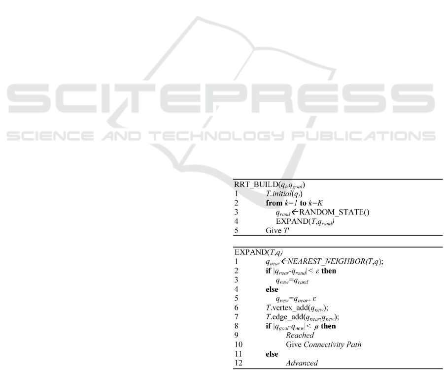
Original RRT (LaValle and Kuffner, 1999; Kuffner
and LaValle, 2000) aims to find a path between initial
(q
i
) and goal (q
goal
) states by growing a tree (T) from
one of these, according to the algorithm in Figure 1.
For this first algorithm, assuming that configuration
space (C) is the same as state space (Q), Q
free
is
defined as obstacle free space, i.e. Q\Q
obs
. Here, it is
a necessity to predefine Q
obs
, q
i
and q
goal
. The
randomized point in Q, q
rand
, finds its nearest point
from the set of vertices, q
near
. If the distance between
these two points is less than some constant distance ε,
then q
rand
becomes q
new
and directly connects to q
near
.
If not, a new ε-long edge is generated between q
near
and q
new
in the direction of q
rand
. This expansion
visualized in Figure 2 continues until an added new
state gets close enough to q
goal
. In case of there is no
solution computation time or number of iterations
must be restricted. As algorithm works randomly, it
could be given a second chance to find a path, or if
there is a possibility of processing, the code can be
run at the same time for more than one tree
independent of each other. The NEAREST-
NEIGHBOR function in the algorithm searches the
closest vertex from the set of vertices to the random
point according to an appropriate distance metric, e.g.
Euclidean, Manhattan and Minkowski distances
(Amato et al., 2000). This process can be accelerated
by using approximate nearest neighbor (ANN)
algorithms.
Figure 1: Basic RRT algorithm.
Time-optimal Smoothing of RRT-given Path for Manipulators
407
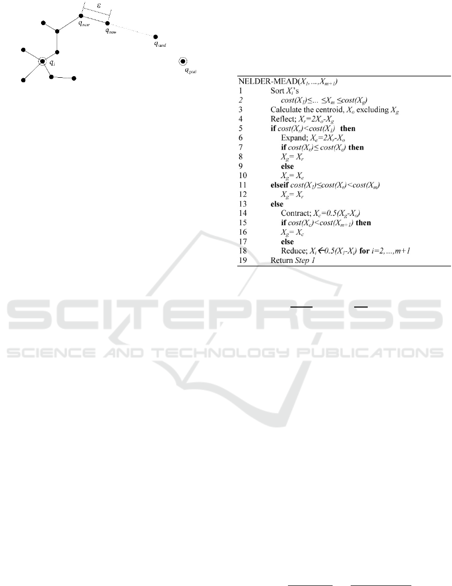
Figure 2: The expand operation.
2.2 Time-optimal Cubic Polynomial
Joint Trajectories
Should the viapoints belonging to a path be obtained
in one way or another, a post-processing is necessary
for the movement to be smooth. There are several
methods for smoothing that is supposed to bring
continuity not only for position but also for velocity
and acceleration. If the position were to be obtained
by cubic functions, obviously, velocity will be
expressed with quadratic, and acceleration with linear
functions. Jerk, on the other hand, will be constant. If
the position and time of the viapoints, and the velocity
and acceleration of the first and last positions, i.e.
boundary conditions, are known, smoothness can be
achieved in the trajectory by defining a cubic position
function, that is piecewise cubic polynomial between
consecutive viapoints. For this to happen, the
position, velocity and acceleration values of the cubic
functions defined in the two consecutive time
intervals should be the same at the viapoint where
they intersect. Based on this fact, before the
emergence of RRT, a methodology for the
formulation and optimization of cubic polynomial
joint trajectories is described in (Lin et al., 1983)
which calls Nelder-Mead Method (Nelder and Mead,
1965), a direct search method of optimization.
Nelder-Mead Method gets to work by suggesting
m+1 number of possible vertices for a cost function
dependent on m variables. Then, those vertices are
sorted according to their cost, and the vertex with the
greatest cost is called X
g
. The X
g
at each iteration is
replaced by a vertex of less cost. The process
described in Figure 3 continues until the cost of X
g
becomes nearly equal to the smallest cost of the
current vertices.
For trajectory planning, let’s take a situation for one
joint, where we have the boundary conditions in the
time interval [t
1
,t
n
], and the information of the
position [q
1
,q
2
,…,q
n-1
,q
n
], and time [t
1
,t
2
,…,t
n-1
,t
n
] at
the n number of knots. There are n-1 known time
intervals, [h
1
,h
2
,…,h
n-2
,h
n-1
] where h
i
=t
i+1
-t
i.
On the
other hand, n-2 accelerations,[
,…,
], are
unknown. A piecewise linear acceleration function,
Q
i
ꞌꞌ(t), which is the second derivative of trajectory
function Q
i
(t) can be written as in (1) for every time
interval h
i
. Clearly, Q
i
ꞌꞌ(t
i+1
)= Q
i+1
ꞌꞌ(t
i+1
) for i=1,…,n-
2 which are also the unknown accelerations. With the
equations from initial and final accelerations, there
will be n linear equations for n-2 unknowns.
Figure 3: Psuedocode for Nelder-Mead Method.
(
)
=
(
)
+
′′(
),
for
≤≤
(1)
Lin et al. (1983) suggest adding two free knots, q
2
and q
n-1
where they reuse n to express the total
number of knots including the extra ones. This
approach provides enough freedom to solve the
system of equations and promises solution
uniqueness.
Later in the same paper (ibid.), assuming time
intervals as cost variables, Nelder-Mead Method is
called. Here, the objective function is the total time,
i.e. sum of time intervals. For the given joint
positions, n feasible trajectories are suggested where
a feasible trajectory respects the kinematic
constraints. Initial vectors of time intervals,
,…,
can be derived from Xꞌ as indicated in (3) where Xꞌ is
the lower bound of the vector of time intervals,
is
the feasible vertex converted from Xꞌ and d
i
’s are
some distance vectors. An estimation for Xꞌ is given
in (2) where j is the joint number, VC
j
is the velocity
constraint for joint j and q
ij
is the position at t
i
.
=
[
ℎ
,ℎ
,…,ℎ
]
=[max
−
,…,
−
()
]
(2)
=
+
(3)
ICINCO 2016 - 13th International Conference on Informatics in Control, Automation and Robotics
408
Lastly, the paper (ibid.) introduces the feasible
solution converter (FSC) which converts an infeasible
vector of time intervals to a feasible one. After
obtaining from (4)-(7) where
and
are the
acceleration and jerk constraints for joint ,
respectively; FSC replaces time intervals by
[ℎ
,ℎ
,…,ℎ
] and accelerations by [
/
,
/
,…,
()
/
], for =1,2,…, where
is the number of joints. What we do here is just
scaling the trajectory.
=max
max
∈
[
,
]
∀
(
)
/
(4)
=max
max
∈
[
,
]
∀
(
)
/
(5)
=max
max
∈
[
,
]
∀
(
)
/
(6)
=max(1,
,
⁄
,
⁄
)
(7)
2.3 Smoothing RRT Results with Cubic
Splines
As mentioned above, while the basic RRT algorithm
gives a path from an initial point to a goal point,
another study (ibid.) can fit a smooth curve for a given
path with boundary conditions and kinematic
constraints. We first suggest using the basic RRT
planner in the configuration space. The state vector,
Q, consists of joint variables. Instead of transferring
the goal point to the configuration space, µ is defined
which is the position tolerance for the goal position
and calculated as the Euclidean norm of deviations in
3 axes. The distance tolerance creates a spherical goal
region with a radius of µ. If the randomized tree
extends into the tolerance region, the exploring stops.
Traditionally, Euclidean distance is selected as the
metric for the nearest neighbor algorithm.
For the curve fitting, as suggested by (ibid.),
=
[
,
,
,
,…,
,
] is calculated as in (8) where
,
and D are determined according to (9-11). Here,
[ℎ
,ℎ
,…,ℎ
] are the elements of
.
,
=
,=
+1
,≠
+1
(8)
=
√
2
(
−1
)
(
√
+−2)
(9)
=
√
2
(
−1
)
(
√
−1)
(10)
=10min
0.2
(
ℎ
−ℎ
)
,
(
ℎ
−ℎ
)
,…,
(
ℎ
−ℎ
)
(11)
During the process summarized in Figure 4, the
newly calculated vertexes will replace the costly
ones. The criteria for the searching to be found
adequate and to stop is determined heuristically.
Figure 4: An approach to time-optimal smoothing of RRT-
given path.
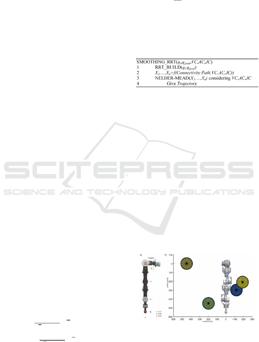
3 SIMULATION AND RESULTS
The code for the RRT algorithm and optimization of
a given path with cubic splines is written in Matlab.
As a manipulator, ITECH humanoid robot arm which
has the six revolute joints given in Figure 5(a), has
been dealt with. Denavit-Hertenberg (D-H)
parameters and link limits of the robot are given in
Table 1; and Table 2 shows the velocity constraints
for all of the joints. Acceleration and jerk constraints
are 100
degrees/sec
2
and 100
degrees/sec
3
,
respectively. In the environment, there are predefined
spherical obstacles with a radius of 75 mm at the
points [200 450 75.5], [450 0 150], [-190 210 400]
and [-120 300 -400] in mm. These obstacles have
been randomly appointed. Initial configuration for the
simulation is [q
1i
, q
2i,
q
3i,
q
4i,
q
5i,
q
6i
]=[90,0,0,0,0,0] in
degrees and the goal position is [-125 0 690] in mm.
The right side view of the initial placement is given
in Figure 5(b).
Figure 5: a) ITECH humanoid robot arm. b) Initial
placement of obstacles and the manipulator.
Time-optimal Smoothing of RRT-given Path for Manipulators
409
The code will work under all circumstances, and
yield a solution if there is one. All of the computations
were done using a laptop with a dual core processor
at 2.4 GHz and 12 GB of RAM. The program has
been run 100 times and always found a different
solution. One of the solutions will be presented as the
illustrative example.
Table 1: D-H parameters and link limits of the robot arm.
j a
j
[mm] α
j
[rad] d
j
[mm] θ
j
[rad] limits [rad]
1 0 - π/2 75.5 θ
1
* -π ̶ + π
2 0 π/2 0 θ
2
*+ π/2
-π/12 ̶ + 2π/3
3 0 - π/2 225 θ
3
*
-π ̶ + π
4 0 π/2 0 θ
4
*
-2π/3 ̶ + 2π/3
5 0 - π/2 214 θ
5
*
-π ̶ + π
6 166.31 0 0 θ
6
*- π/2 -2π/3 ̶ + 2π/3
Table 2: Velocity constraints of the robot arm.
joint, j 1 2 3 4 5 6
velocity (
o
/sec) 20 20 40 40 60 60
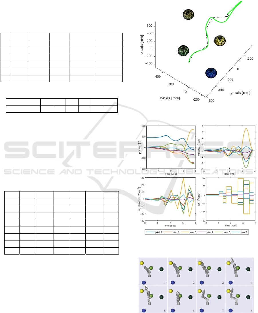
Viapoints given by RRT algorithm is given in
Table 3 and shown in Figure 6. As might be expected,
these are completely random points in Q
free
. For
smoothing, Xꞌ and
are calculated as:
Xꞌ = [0.0065 0.0065 0.0072 0.0060 0.0318 0.0095
0.0113 0.0434 0.0434]
= [0.1995 0.1995 0.2206 0.1836 0.9741 0.2919
0.3454 1.3313 1.3313]
Table 3: RRT-given joint configurations.
j
1 [
o
] 2 [
o
] 3 [
o
] 4 [
o
] 5 [
o
] 6 [
o
]
knot 1 90 0 0 0 0 0
knot 2 94.04 -14.91 4.29 -10.01 6.38 1.50
knot 3 102.28 -14.24 -1.33 -19.53 8.19 -11.21
knot 4 109.14 -18.78 -6.41 -25.75 20.54 -12.85
knot 5 72.73 -46.16 -44.15 -28.50 33.89 -6.06
knot 6 64.89 -54.08 -22.33 -32.21 18.73 -18.80
knot 7 77.80 -63.96 -29.63 -44.53 5.90 -33.01
knot 8 -21.70 -143.59 166.45 -67.69 -152.31 0.01
Hence; D, δ
1
and δ
2
are obtained by the help of (9-11)
as 0.9823, 0.8615 and 0.1669, respectively. After the
optimization process, the optimized vector of time
intervals, X
opt
, is computed as
X
opt
= [0.0908 0.9278 0.2367 0.2040 0.4296
0.4943 0.4359 0.5767 0.3503]
i.e. the optimum total time is 3.7462 seconds. As it is
seen in Figure 7, boundary conditions and kinematic
constraints are respected while trajectory planning.
Lastly, Figure 8 shows the motion frame by frame.
Since cubic splines are preferred for the smoothing,
there is an inevitable motion resembling a loop.
Hence, the results can be considered as time-optimal
only for cubic spline trajectories.
Figure 6: RRT-given path (dashed line) and smoothed path
(green line) for the end-effector of the robotic arm.
Figure 7: Jerk, acceleration, velocity, and position profiles
of the trajectory.
Figure 8: Eight consecutive frames of the motion of robot
simulated with SimMechanics toolbox of Matlab.
ICINCO 2016 - 13th International Conference on Informatics in Control, Automation and Robotics
410

4 CONCLUSIONS
The smoothing of RRT-given paths is a topic still
being studied. In this study, firstly, for a 6 degrees of
freedom manipulator, a connectivity path has been
determined with a sampling-based path planning
algorithm, RRT, which has been popular for the last
two decades. Following this, for path smoothing,
Nelder-Mead Method based time optimization
method of joint trajectories, which has been
suggested by Lin et al., has been used. This
adaptation, in addition to other smoothing practices
(Hauser and Ng-Thow-Hing, 2010; Lau and Byl,
2015), has jerk limitation and time optimization
advantages. The program has been run repeatedly for
a set-up where there is at least one solution, and each
time a feasible solution has been found.
Dynamic issues such as the required torques for the
motion, dynamic stability and control of the
manipulator have not dealt with in this study. It is
being considered to make a motion planning using
kynodynamic RRT algorithm as future work. Our
approach can also be implemented for the RRT*
optimized algorithm. In the RRT-given path
optimization, Nelder-Mead Method can be compared
to other algorithms. Lastly, the plan is to test the
approach on the manufactured robot.
ACKNOWLEDGEMENTS
This study is partially supported by Scientific
Research Projects Unit of Istanbul Technical
University (Grant No.38826). The authors wish to
thank Cihat Bora Yigit for his time and comments on
the paper.
REFERENCES
Amato, N., Bayazit, O., Dale, L., Jones, C. and Vallejo, D.
(2000). Choosing good distance metrics and local
planners for probabilistic roadmap methods. In: IEEE
Transactions on Robotics and Automation. pp.442-447.
Barraquand, J., Langlois, B. and Latombe, J. (1991).
Numerical potential field techniques for robot path
planning. In: IEEE Transactions on Systems, Man and
Cybernetics, vol. 22, no. 2. pp.224-241.
Bertram, D., Kuffner, J., Dillmann, R. and Asfour, T.
(2006). An Integrated Approach to Inverse Kinematics
and Path Planning for Redundant Manipulators. In:
IEEE International Conference on Robotics and
Automation. pp.1874-1879.
Boyacioglu, B. and Ertugrul, S. (2015). Obstacle Avoided
Trajectory Planning of a 6 DOF Humanoid Robot Arm.
In: 2nd Conference of Robot Science in Turkey.
Canny, J. (1988). On the complexity of kinodynamic
planning. Ithaca, NY: Cornell Univ., Dep. of Computer
Science.
Diankov, R., Ratliff, N., Ferguson, D., Srinivasa, S. and
Kuffner, J. (2008). BiSpace Planning: Concurrent
Multi-Space Exploration. In: Robotics: Science and
Systems IV.
Güleç, M. and Ertugrul, S. (2014). Design and Trajectory
Control of a Humanoid Robot Arm. In: Turkish
Automatic Control Conference. Istanbul, pp.90-95.
Hauser, K. and Ng-Thow-Hing, V. (2010). Fast Smoothing
of Manipulator Trajectories using Optimal Bounded-
Acceleration Shortcuts. In: IEEE International
Conference on Robotics and Automation. pp.2493-
2498.
Kavraki, L., Švestka, P., Latombe, J. and Overmars, M.
(1996). Probabilistic roadmaps for path planning in
high-dimensional configuration spaces. In: IEEE
Transactions on Robotics and Automation, vol 12, no.
4. pp.566-580.
Kuffner, J. and LaValle, S. (2000). RRT-Connect: An
Efficient Approach to Single-Query Path Planning. In:
IEEE International Conference on Robotics and
Automation. pp.1-7.
Lau, C. and Byl, K. (2015). Smooth RRT-Connect: An
extension of RRT-Connect for practical use in robots.
In: IEEE International Conference on Technologies for
Practical Robot Applications. pp.1-7.
LaValle, S. and Kuffner, J. (1999). Randomized
Kinodynamic Planning. In: lEEE International
Conference on Robotics & Automation. pp.473-479.
Lin, C., Chang, P. and Luh, J. (1983). Formulation and
optimization of cubic polynomial joint trajectories for
industrial robots. IEEE Transactions on Automatic
Control, 28(12), pp.1066-1074.
Nelder, J. and Mead, R. (1965). A Simplex Method for
Function Minimization. The Computer Journal, 7(4),
pp.308-313.
Perez, A., Karaman, S., Shkolnik, A., Frazzoli, E., Teller,
S. and Walter, M. (2011). Asymptotically-optimal Path
Planning for Manipulation using Incremental
Sampling-based Algorithms. In: IEEE International
Conference on Intelligent Robots and Systems.
pp.4307-4313.
Shkolnik, A. and Tedrake, R. (2009). Path planning in
1000+ dimensions using a task-space Voronoi bias. In:
IEEE International Conference on Robotics and
Automation. pp.2061-2067.
Weghe, M., Ferguson, D. and Srinivasa, S. (2007).
Randomized Path Planning for Redundant
Manipulators without Inverse Kinematics. In: IEEE-
RAS International Conference on Humanoid Robots.
pp.477-482.
Time-optimal Smoothing of RRT-given Path for Manipulators
411
