Dynamic Model-based Control of Redundantly Actuated,

Non-holonomnic, Omnidirectional Vehicles

Christoph St¨oger, Andreas M¨uller and Hubert Gattringer

Institute of Robotics, Johannes Kepler University Linz, Altenberger Straße 69, 4040 Linz, Austria

Keywords:

Dynamic Modeling and Control, Redundant Actuation, Pseudo-omnidirectional, Singularities.

Abstract:

Vehicles with several centered orientable wheels have one of the highest maneuverability and are hence an

excellent choice for transportation tasks in narrow environments. However, they are non-holonomic, in general

redundantly actuated, and additionally suffer from conﬁguration singularities, which makes their modeling and

control challenging. Existing control approaches only consider the vehicle kinematics whereas the required

torques are commonly controlled by classical PD motor controllers. However, this leads to considerable

tracking errors and a violation of the constraints especially during acceleration phases. Moreover, actuator

counteractions and an undeﬁned torque distribution can be observed. This paper introduces a model-based

control concept that overcomes these issues. It resolves counteractions and distributes torques according to

physical limitations which signiﬁcantly reduces slippage and the energy consumption and further reduces the

tracking error. To this end, an inverse dynamics solution of a redundantly parametrized model is used. The

method is robust to conﬁguration singularities. This is conﬁrmed by experimental results.

1 INTRODUCTION

Mobile platforms offer a large workspace for appli-

cations in service robotics as well as manufacturing.

Their main application is, especially in industry, still

the transportation of goods –a seemingly simple task

that can, however, become very complex given the

demand from industry for compact and cost-efﬁcient

shop ﬂoor solutions. A consequence is that a pre-

cise locomotion with a mobile base offering the max-

imum degree of maneuverability δ

(Campion et al.,

1996), i.e. δ

= 3, is ever more relevant. Vehicles

with δ

= 3 are also called omnidirectional since they

are able to move in each direction and independently

change their orientation. Holonomic omnidirectional

vehicles, equipped with n ≥ 3 Mecanum or Swedish

wheels, are the most popular type of this class. They

need a small number of actuators, since they do not

need to steer, and are easy to control. However,

Mecanum wheels possess poor load capacities com-

pared to standard wheels, they introduce vibrations

to the actuators and chassis, and lead to much higher

slippage. Platforms with n ≥ 2 centered orientable

standard wheels overcome these problems. Center

orientable wheels are wheels which can be steered

about a vertical axis passing through the center of the

wheel. Such platforms are omnidirectional as well but

non-holonomic,i.e. they can independently attain any

position and orientation but may have to reorient their

wheels during the navigation. For this reason they are

often called pseudo-omnidirectional.

The number of driven wheels depends on the

transporter size, i.e. the payload, and is often higher

than 2. The driving motors are thereby acting in par-

allel which means that the vehicle is not only non-

holonomic but also redundantly actuated. There are

several publications about the higher-level kinematic

control of such vehicles (Giordano et al., 2009; Of-

tadeh et al., 2013; St¨oger et al., 2015), which results in

a feasible motion of the wheels and moves the vehicle

to a destination. However, there is hardly any lower-

level dynamic control scheme for actually achieving

this motion reported in the literature. It is mostly in-

dicated that a simple PD controller is used. Such a

control neither takes the dynamic of the vehicle into

account, nor the redundancy of the actuation. Consid-

erable errors in dynamic phases and unnecessary high

torques due to the actuator counteraction, which again

lead to slip, are the consequence.

Common approaches for controlling platforms

with δ

< 3 can be divided into two classes: 1) ro-

bust control and 2) model-based control strategies. In

the ﬁrst class sliding mode controllers are widely used

(Yang and Kim, 1999). One and the same controller

Stöger, C., Müller, A. and Gattringer, H.

Dynamic Model-based Control of Redundantly Actuated, Non-holonomnic, Omnidirectional Vehicles.

DOI: 10.5220/0005980200690078

In Proceedings of the 13th International Conference on Informatics in Control, Automation and Robotics (ICINCO 2016) - Volume 2, pages 69-78

ISBN: 978-989-758-198-4

works for different loads quite well but the robust-

ness has to be paid by a high switching frequency of

the input torques. Thereby, the second class is more

promising for us. A model-based inverse dynam-

ics controller reduce the tracking error signiﬁcantly

and can easily be adapted if the load of the vehicle

changes. So far there is hardly any dynamic con-

trol method for redundantly actuated platforms with

= 3. In (Lee and Li, 2015) the authors use the in-

verse dynamics solution extended by a sliding mode

controller but have not addressed the redundancy res-

olution or counteraction avoidance. Methods for the

control of redundantly actuated systems can be found

in the ﬁeld of parallel mechanisms (M¨uller and Huf-

nagel, 2012) and are adapted in this paper to the needs

of mobile robots. Our aim is to use only a minimal de-

mand of torque and to distribute this demand among

the actuators by considering their limitations as well

as differences in frictional conditions, e.g. due to an

unbalanced load, in order to increase the uptime of the

vehicle and reduce slippage in the resulting motion.

The result is a novel concept for the low-level control

of non-holonomic,omnidirectional vehicles equipped

with an arbitrary number n of wheels. The control

concept can be seen as building block which is inde-

pendent from the higher-level control scheme used for

motion planning.

Although there is a large number of dynamic mod-

els for other platform types, e.g. differential drives

(Fukao et al., 2000) or car like systems (De Luca

et al., 1998), only a few models are available for

omnidirectional, non-holonomic vehicles. Moreover,

those models either do not consider constraint forces

(Lee and Li, 2015) or neglect the wheels (Ploeg et al.,

2002) which results in a considerable model error.

However, such models can still be found in the lit-

erature since they bypass the resolution of the singu-

lar rolling constraints. Therefore, a novel dynamic

model is presented in this paper. It is redundantly

parametrized, which is especially also valid in sin-

gular conﬁgurations, and includes all relevant effects.

Constraining forces are numerically eliminated by a

null space projection method (M¨uller and Hufnagel,

2012). The null space projector is computed by a

novel semi-analytic orthogonalization method which

takes the structure of the constraints into account and

is computationally efﬁcient. The latter is especially in

the context of the control crucial.

The paper is structured as follows. In Section

2 the description of the platforms kinematics is pre-

sented. The conﬁguration variables are described and

the rolling constraints are formulated. In Section 3

the redundant parametrized dynamic model is derived

whereby an overview about the modeled effects in-

cluding friction is given and the constraint forces are

eliminated. In Section 4 the inverse dynamics is com-

puted and the torque distribution method presented.

Subsequently, the control concept is formulated and

its asymptotic stabilization is proofed. Experiments

which validate the theory are presented in Section 5.

The paper closes with a summary in Section 6 and

some remarks for future research.

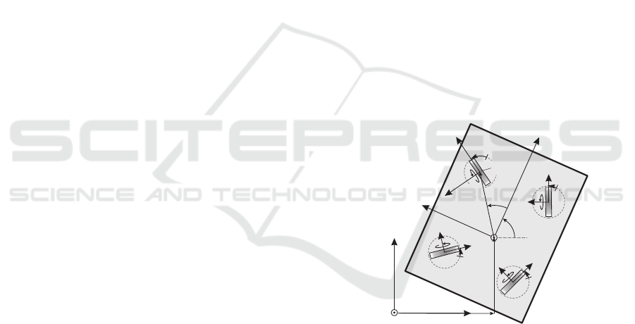
2 PLATFORM KINEMATICS

The variables that parametrize the current conﬁgura-

tion of the platform, see Figure 1, can be divided into

two sets (Ostrowski and Burdick, 1996). The ﬁrst set

describe the vehicle’s posture, i.e. displacement of

the chassis-ﬁxed frame F

= {O

y} relative to

an inertial frame F

= {O

y}.

Assumption 1. The vehicles motion is assumed to be

restricted to the horizontal plane.

With Assumption 1 the pose can be parametrized us-

ing q

= (x,y,γ)

∈ SE(2). The vector (x,y) ∈ R

describes the reference point O

in the frame F

and

γ ∈ S

is the angle enclosed by

x and

chassis

Figure 1: Non-holonomic, omnidirectional vehicle with n =

4 centered orientable wheels.

The second set of variables are called shape or inter-

nal variables. They describe the conﬁguration of the

locomotion system and are given by n roll angles ϕ

and n steer angles ϕ

, with i ∈ {1, .. .n}. They are

summarized in

= (ϕ

,... ϕ

,ϕ

,... ϕ

)

∈ T

. (1)

Here T

is the 2n dimensional torus. For later pur-

pose additional frames F

= {O

y} are at-

tached at each drive unit.

The conﬁguration of the mobile platform is thus de-

scribed by the vector of generalized coordinates

q = (q

)

∈ Q = SE(2) × T

. (2)

ICINCO 2016 - 13th International Conference on Informatics in Control, Automation and Robotics

Although ideal rolling is a simpliﬁed assumption

we can use it within the control in order to minimize

the resultant slippage and counteraction. Ideal rolling

means that the longitudinal velocity (

x direction) of

a certain wheel i is consistent with its rolling speed,

which requires

cos(ϕ

+ γ)˙x+ sin(ϕ

+ γ)˙y+ l

sin(ϕ

− ϕ

)

γ− r

= 0, (3)

and that the lateral velocity (

y direction) is zero, i.e.

−sin(ϕ

+γ) ˙x+cos(ϕ

+γ) ˙y+l

cos(ϕ

−ϕ

)

γ = 0.

(4)

The polar coordinates l

and ϕ

describe the position

of the ith wheel O

observed from F

, see Figure 1.

The following properties directly follow from the

rolling constraints, see Equation (3) and (4):

Property 1. The constraints can be written in Pfaf-

ﬁan form, i.e. linear in velocities, as J

J(q

q = 0.

Property 2. The n steering velocities

are uncon-

strained. Hence, the columns of J

J which correspond

to them are zero.

The rank m of J

J ∈ R

2n,3+2n

determines the number

of independent constraints. Hence, the number of in-

dependent velocities respecting the constraints, also

referred to as generalized velocities, is

= 3 + 2n− m. (5)

Another interesting property is that the n lateral con-

straints (4) only restrict the chassis twist ( ˙x, ˙y,

γ). By

considering the corresponding rows in J

J, one can eas-

ily proof the following property.

Property 3. The number and set of independent lat-

eral constraints depends on the steering angles and is

between 1 and 3.

In the case of n > 2 wheels the minimum number of

generalized velocities is δ

= 3 + 2n − (n + 3) = n.

Referring to Property 2, they are given by the uncon-

strained steering angles. In this case, the vehicle can

not drive but only steer the wheels. Thus, vehicles

with n > 2 wheels have to drive in regions of reduced

rank. In this regions, only one particular twist, namely

the rotation about the instantaneous center of rotation,

is possible. Some wheel setups, especially for n = 2

wheels, permit the axial alignment of all wheel axes.

In this special conﬁguration, the number m of inde-

pendent constraints further reduces by 1 since all lat-

eral constraints are equal. Such conﬁgurations allow

the vehicle to rotate about an arbitrary point on the

line speciﬁed by the wheel axes. This is summarized

by the following property.

Property 4. The constraint matrix J

J is either perma-

nent singular or can become singular. The number of

generalized velocities is thus δ

∈ {n+ 1,n + 2}.

3 DYNAMIC MODELING

3.1 Redundantly Parametrized

Equations of Motion

The equations of motion are derived using the Projec-

tion Equations

∑

b=1

∂

c,b

∂



c,b

IR R

c,b

−

c,b

IR R

−



= 0.

(6)

Projection Equations are based on the Newton-

Euler equations for body b which are evaluated in a

reference frame F

, and are projected onto the direc-

tion of the generalized coordinates q

q. Here

c,b

is the linear momentum of the center of grav-

ity (c) of body b.

is the angular mo-

mentum, and

c,b

and

are corresponding trans-

lational and angular velocities.

ω is a skew symmet-

ric matrix representing the cross product

ωp

p = ω

ω× p

c,b

and

are total forces and torques acting on

the center of gravity / body. The Equations (6) are

used to model inertia effects, the inﬂuence of traction

and friction forces as well as motor torques.

Inertia is considered for N = 2n + 1 bodies:

• the chassis (c)

and n drive units including:

• n steer motors (si), which are mounted on the

chassis and are rigidly coupled with a drive unit

• n drive motors (ri), which are in turn mounted

on the drive unit and are rigidly coupled with the

wheel.

The inertia of the chassis is, in general, signiﬁcantly

higher than the inertia of the drive unit. However,

since especially the orientation of the drive unit has

a much higher acceleration they are relevant too. The

velocities of the chassis are

c,c



˙xcos(γ)+ ˙ysin(γ) − ˙xsin(γ) + ˙ycos(γ) 0





0 0



and the velocities of the steer axes and the rolling

wheels are

c,si

c,ri





˙xcos(γ+ ϕ

) + ˙ysin(γ+ ϕ

) + l

sin(ϕ

− ϕ

)

− ˙xsin(γ+ ϕ

) + ˙ycos(γ+ ϕ

) + l

cos(ϕ

− ϕ

)







0 0

γ+





γ+



Dynamic Model-based Control of Redundantly Actuated, Non-holonomnic, Omnidirectional Vehicles

all vectors are expressed in F

(Figure 1). It is as-

sumed that the center of gravity of the drive unit co-

incides with the steering axis O

There are two kinds of friction sources. The ﬁrst

kind is bearing friction. It is commonly modeled as

a viscose and coulomb friction using a static model

(Bona and Indri, 2005). The model is computationally

inexpensive and the parameters can be easily identi-

ﬁed since the model is linear w.r.t. the parameters.

The second kind of friction source is the tire/soil con-

tact. Since ideal rolling is assumed the generalized,

i.e. projected, traction forces Q

are imposed by the

constraints (3), (4):

= J

λ, (7)

where λ

λ ∈ R

are the corresponding Langrange mul-

tipliers. The ground contact model must also take the

rolling resistance into account. The rolling resistance

is caused by elastic deformation of tire and soil, and

can again be modeled (within a certain velocity range)

by a Coulomb and viscous friction model (Hall and

Moreland, 2001). The applied driving (r) and steering

(s) torques are given by



0 0 1



(τ

− µ

sci

sign(

) − µ

svi

)



0 1 0



(τ

− µ

rci

sign(

) − µ

rvi

where µ are friction coefﬁcients for the Coulomb (c)

and viscous (v) friction, τ

is the steering torque and

the rolling torque, respectively. The discontinuous

sign(x) function leads to chattering about zero veloc-

ity. In order to avoid that, this function is replaced in

the control law by the smooth tanh(x/ε) function. The

parameter ε is used to determine the region where the

force is reduced due to low speeds. The value of ε de-

pends on the application. In the experiment it was set

to 0.01rad/s, which corresponds to a driving speed of

≈ 1mm/s for the considered system.

The dynamics of the non-holonomic, omnidirec-

tional vehicle can be expressed by the system of dif-

ferential algebraic equations

M(q

q+C

C(q

q+ f

q) = B

B(q

q)u

u+J

J(q

λ (8a)

J(q

q = 0. (8b)

Here M

M ∈ R

2n+3,2n+3

is the generalized inertia ma-

trix, C

q ∈ R

2n+3

includes Coriolis and centrifugal

forces, f

f ∈ R

2n+3

Coulomb and viscous friction, u

u =



,... τ

,τ

,... τ



∈ R

, and B

B ∈ R

2n+3,2n

are

the input torques and matrix, and J

λ the generalized

constraining forces acting on the system.

Assumption 2. It is assumed that each wheel is fully

actuated, i.e. each wheel has a steering and driving

motor.

Then, the input matrix has the following structure

B =



n+3,n

n,n+3

n,n



(9)

where 0

i, j

∈ R

i, j

is a zero matrix, I

n,n

∈ R

n,n

a identity

matrix and



3,n

n,n



. (10)

The dimensions slightly change for vehicles where

this is not the case but the method is still valid.

3.2 Elimination of Constraint Forces

The Equations (8) form a differential algebraic sys-

tem, and their evaluation requires the determination

of the Lagrange multipliers λ

λ. The computational ex-

pense of this computation is in particular problematic

since it should be used within the control law (M¨uller

and Hufnagel, 2012). Therefore, the constraint reac-

tions are not computed but eliminated instead. This

is commonly done by reformulating the equations of

motion with a set of generalized velocities that respect

the constraints. However, the subset of regular con-

straints depends on the conﬁguration of the vehicle.

As a consequence, a set of different generalized ve-

locities and their corresponding dynamics equations

are often used. However, this leads to issues dur-

ing the transition between these models which can be

avoided by the following approach.

(M¨uller and Hufnagel, 2012) suggest to use one

redundantly parametrized model, as in (8), but elimi-

nate the constraining forces by projecting the dynam-

ics equation with a projector N

N to the null space of J

This projector is not unique. The requirements are

N = 0, (11)

i.e. N

N is an orthogonal complement of J

J, and

rank(N

N) = δ

, i.e. N

only removes constraining

forces. Projecting Equations (8) leads to

q+C

q+ f

f) = N

u. (12)

There are two methods proposed by (M¨uller and

Hufnagel, 2012) for the analytic computation of N

Both, however assume regular constraints and, as a

consequence of Property 4, are not directly applicable

for pseudo-omnidirectional vehicles. In this work a

semi-analytical approach is used which consist of an

analytical and a numerical step.

In the analytical step Property 2 is used

to determine n columns of N

N. The columns

k ∈ {4 + n,. .. 3 + 2n}, corresponding to the

steering velocities, of J

J are zero. Hence, unit

vectors u

, which are zero but have 1 at the

kth component, lie in the null space of the

ICINCO 2016 - 13th International Conference on Informatics in Control, Automation and Robotics

Algorithm 1: Gram-Schmidt inspired projec-

tion method for the null space computation. k·k

is the Euclidean vector norm.

1 Function compute remaining null space vectors

input : Constraint matrix J

output: Remaining null space directions N

2 K

K = [J

], N

= [ ], i = 1

3 δ

= n

4 for i = 1,... 3 do

q = u

6 i = i+ 1

7 eliminate

directions(

q, K

8 if k

qk > ε then

q =

q/k

10 N

= [N

11 δ

= δ

+ 1

12 K

K = [K

13 end

14 end

15 end

16 Function eliminate

directions

input :

q vector under consideration, K

K column

vectors represent directions which

should be eliminated

output: n

n: remaining components of

17 k = 1

18 repeat

19 j

j = column(K

K, k)

20 k = k + 1

q =

q−





22 until k

qk < ε or k >nr

of columns(K

23 end

constraint Jacobian, i.e. J

= 0. Hence, the full rank

matrix



n+3,n

n,n



(13)

satisﬁes (11). This provides n columns of N

In the numerical step the remaining δ

− n null

space vectors are computed. This is commonly done

by a singular value or full QR decomposition. These

algorithms, however, compute a basis for both, the

n + 2 (or n + 1) constrained and the remaining 1 (or

2) unconstrained directions and thereby add an un-

necessary high computational expense to the method-

ology. An algorithm that avoids this is introduced in

the following, see Algorithm 1. It is inspired by the

Gram-Schmidt orthogonalization (Bj¨orck, 1994).

The algorithm determines a non-trivial vector

which is orthogonal to the constrained directions j

where j

j is a transposed row of J

J and hence again

fulﬁlls J

= 0. The search starts with

q = u

(1,0, .. . 0)

that correspond to a pure translation in

the x-direction of frame F

, see Figure 1 and (2). The

rolling constraints are obviously violated since the en-

tries that correspond to the drive velocities

are

zero. However, since the column space of J

and the

allowed directions form an orthogonal complement,

this vector can always be split into allowed and con-

strained components. The constrained components

are removed in the elimination

directions phase by

means of a vector projection. This reveal whether

there is any motion possible which has a component

in the x-direction. If not, the y-direction or ﬁnally a

pure rotation is tried. The algorithm also works in

the case of aligned wheel axes, i.e. 2 missing vectors.

The only thing to do is to continue searching after one

admissible velocity is found, and to remove not only

the constrained directions but also the former found

admissible directions.

The computation is very efﬁcient since the projec-

tion, which is needed for the elimination step, only

consists of simple arithmetical operations and the

number of projections is limited to 6n. J

J has only

zero columns in the last n entries, thus the result has

the following structure



n,δ

−n



(14)

where N

∈ R

n+3,δ

−n

is computed by the algorithm,

so that the columns of N

are orthonormal.

Combining the analytical N

and numerical N

null space bases ﬁnally result in

N =







n+3,n

n,δ

−n

n,n



. (15)

Property 5. The columns of the null space projection

matrix N

N are orthonormal. Hence the left inverse of

N is given by its transposed.

4 MODEL-BASED CONTROL

4.1 Inverse Dynamics and Redundancy

Resolution

At this point the inverse dynamics can be computed

by evaluating (12) with a desired motion q

(t)

f = Q

= N

, (16)

which determines the required generalized forces Q

Resolving the last term in (16) yields required torques

thus solving the inverse dynamics problem. The

computational effort of this task can be signiﬁcantly

reduced if the structures of B

B, see (9), and N

N, see (15),

are taken into account



−n,n

n,n+3

n,n







r,d

s,d



. (17)

Dynamic Model-based Control of Redundantly Actuated, Non-holonomnic, Omnidirectional Vehicles

Hence, the special choice of N

N decouples the driving

and steeringu

torques. The latter are directly given

by the last n elements Q

s,d

of the generalized torques

The driving torques must be computed by the re-

maining equations

= Q

r,d

. (18)

By investigating the dimensions of the projected input

matrix

= N

∈ R

−n,n

, where δ

− n is in gen-

eral 1 or 2, it follows that the equation is underdeter-

mined. Hence, there is an inﬁnity number of driving

torquesu

which result in the sameQ

r,d

. The system is

therefore called redundantly actuated. To resolve this

redundancy, the solution is chosen which minimize

the following quadratic cost function (M¨uller, 2011)

∗

= arg min

(19a)

s.t.

= Q

r,d

, (19b)

with a positive deﬁnite weight matrix W

W ∈ R

n,n

. The

cost function ensures that only a minimal torque de-

mand is used to provide Q

r,d

. The distribution of this

demand can be done by choosing a proper weight ma-

trix. In our approach the following diagonal matrix is

used

W = diag



1/τ

r,max1

,... 1/τ

r,maxn



, (20)

whereby τ

r,maxi

are the maximum torques w.r.t. the

motor and friction limitations. The latter is approxi-

mated by the stall torques, that is the maximum torque

which can be applied to a single wheel, while accel-

erating the chassis against a stop, that does not result

in slippage. They are determined by experiments and

should include frictional differences due to an unbal-

anced load in the torque distribution.

The solution of (19) is given by

= W

−1



−1



−1

{z }

=: B

r,d

. (21)

Where

is a right inverse of B

, i.e. B

= I

n,n

Summarizing, the inverse dynamics yields

= (N

, (22)

with the right inverse



l−n,n

n,n+3

n,n



(23)

of the projected input matrix N

B .

4.2 Augmented PD-control

The inverse dynamics (22) provides the torque needed

to follow a given desired motion q

. However, there

is no feedback stabilization mechanism in this law.

Hence, model uncertainties and disturbances will in-

evitably lead to signiﬁcant errors. The classical ap-

proach to eliminate these errors is a decentralized

strategy which independently controls the 2n actuated

degrees of freedom

= P

(

ri,d

−

)dτ + D

(

ri,d

−

) (24)

= P

(ϕ

si,d

− ϕ

) + D

(

si,d

−

). (25)

The rolling constraints instantaneously only admit

∈ {n + 1,n + 2} independent velocities, hence the

result is a violation of the rolling constraints and a

counteraction of the control torques.

Our approach resolves this problem by a central-

ized model-based control

APD

= (N



(

−

q)+P

(

−

q)dτ



. (26)

The system matrices and vectors M

M,C

C, f

f are evalu-

ated by the vehicles current pose/velocity. The argu-

ments of them are suppressed due to the lack of space.

D,P

P ∈ R

,δ

are positive deﬁnite gain matrices. The

idea behind (26) is to use the projected velocity error

and its integral

= N

(

−

q), e

dτ, (27)

instead of the individual velocity error of each wheel

to stabilize the system. The counteraction is thereby

removed since the dimension of the error is equal to

the local degree of freedom δ

. The resulting torques

are ﬁnally again distributed in a minimal fashion over

the existing drives.

In the following it is proven that (26) asymptot-

ically stabilizes

q along a desired motion

. It is

therefore assumed that the desired velocity

is pro-

vided by a higher-level controller and respects the

constraints. By applying (26) to (12) and project

it into unconstrained directions, the closed loop dy-

namic equations can be formulated as follows

−

q)+N

−

q)+D

= 0. (28)

Moreover,

q and

respect the constraints. Hence,

they are lying in the null space of J

J and, as such, can

be expressed by a linear combination v

of the ba-

sis N

N of this space

−

q = N

−N

= N

. (29)

ICINCO 2016 - 13th International Conference on Informatics in Control, Automation and Robotics

It follows from Property 5 and Equation (27) that e

− v

. Inserting (29) in (28), yields the following

error system

= 0 (30)

with the projected mass matrix

M = N

N and the

projected Coriolis and centrifugal forces

where

C = N

N +N

N. The stability can be proven by

introducing the following Lyapunov function

V =

. (31)

Differentiating V w.r.t. time along a solution

(t),e

(t) of (30) yields

V =

(

M − 2

C)e

−e

= −e

≤ 0. (32)

Thereby, the following properties are used:

Property 6.

M is positive deﬁnite,

Property 7.

M − 2

C is skew symmetric.

The proof of them can be found in (Murray et al.,

1994). Referring to the Krasovskii-LaSalle invari-

ance principle, for a positive deﬁnite function V > 0

with a negative semi-deﬁnite derivative

V ≤ 0 the

state converge to a rest position in the subset of

V = 0. The only rest position of (30) in this subset

is (e

(t),e

(t)) = (0, 0) which proves the asymptotic

stabilization of the control law.

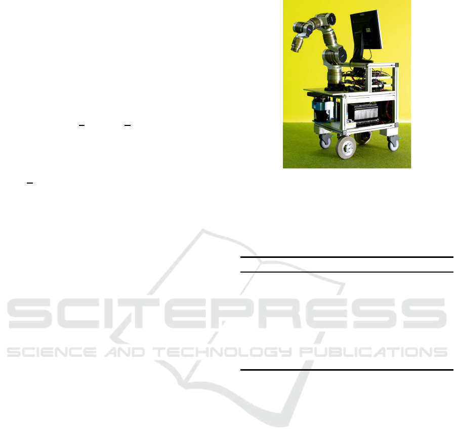
5 EXPERIMENTAL RESULTS

In this Section experimental results of the proposed

theory are presented. The used vehicle is equipped

with n = 2 actuated wheels and is shown in Figure

2. The wheels are diametrically mounted about the

reference point O

. The front wheel is indexed by

i = 1, the rear wheel by i = 2. The driving motors

are DC motors with a maximum torque of 25.6Nm.

They allow a maximum driving speed of 4.1rad/s

which equals a linear velocity of

r = 0.41m/s

with a wheel radius r = 0.1m. The steering motors

are brushless DC motors with a maximum torque of

129Nm and a maximum steering speed of 195.95

◦

/s.

Selected parameters of the considered vehicle are

summarized in Table 1.

Figure 3 visualizes the driven maneuver. It can be

divided into two parts. The ﬁrst part (t = 0.. .5s) is

a pure rotation by γ = 180

◦

about the reference point

. Therefore, the wheel axes have to be aligned,

hence it is a motion where the constraints are singu-

lar. In the second part, a mixed motion with transla-

tional and rotational components is done in a regular

Figure 2: Non-holonomic omnidirectional manipulator with

n = 2 actuated wheels. The laser scanner marks the front

side.

Table 1: Selected parameters of the equations of motion.

Inertias are given together with the corresponding rotation

axes.

symbol value description

93 kg chassis weight

4.51kgm

inertia chassis

z axis

20.5· 10

−3

kgm

inertia steering unit

0.2234kgm

inertia steering unit

rci

0.88 Nm Coulomb, driving

rvi

0.35Nms/rad viscous, driving

sci

2.11 Nm Coulomb, steering

svi

2.08Nms/rad viscous, steering

conﬁguration. The orientation is chosen to be always

tangential to the desired (x

) curve. The corre-

sponding steering and driving velocities are summa-

rized in Figure 4. The motion is ﬁrstly controlled by a

classic PD control approach (25) and secondly by the

proposed model-based control (26). A fair compari-

son between them is ensured by an independent op-

timization of the corresponding control coefﬁcients.

The result of this optimization is summarized in Ta-

ble 2. The coefﬁcients P

and D

corresponds to the

error component which is projected by N

while P

and D

correspond to the projection of N

Since the steering angles are unconstrained and

regularly actuated, both control concepts result in the

same error correction laws. Thus, the same control

coefﬁcients can be used. Differences between the re-

sulting tracking errors, see Figure 6, are a result of the

inverse dynamics and can be primary seen in acceler-

ation phases t ∈ {11,15,. ..18}s. There, the model-

based control result in a signiﬁcantly lower tracking

error. The tracking error of the driving velocities can

Dynamic Model-based Control of Redundantly Actuated, Non-holonomnic, Omnidirectional Vehicles

y in m

x in m

start

0.25

0.5 0.75 1 1.25 1.5 1.75

0.25

0.5

0.75

1.25

1.5

1.75

Figure 3:

replacements

Desired chassis position, sampled chas-

sis orientation and driving direction,

points in time t

∈

{0s,10s, 12s,16s,22s}.

t in s

0 2 4 6

14 16 18 20 22

−1

−0.5

0.5

max

Figure 4: Driving velocity of front and rear wheel

normalized by r

r,max

=0.4m/s, steering velocity of

front and rear wheel normalized by

s,max

=180

◦

/s.

be found for the front wheel i = 1 in Figure 5. Sig-

niﬁcant differences can again mainly be found at ac-

celeration phases t ∈ {0,3,16,20}s. The differences

can also be seen in the total slip distance (constraint

violation)

∆

t=0

∆

longi

∆

lati

dt. (33)

It is computed by integrating the left-hand side of

Equation (3) and (4). Due to violation they are not

zero but equal to some longitudinal

∆

longi

and lateral

∆

lati

slip. Along the 2.595m long path, the model-

based control leads to ∆

+ ∆

= 0.041m (1.58% of

total path length) slip distance, whereby classic PD

control leads ∆

+ ∆

= 0.137m (5.28% of total path

length) slip distance.

Signiﬁcant differences can also be noticed in the

t in s

0 2 4 6 8 10 12 14 16 18 20 22

−40

−30

−20

−10

r1d

−

) in mm/s

Figure 5: Velocity tracking error for the classic PD and

model-based controlled front wheel i = 1.

Table 2: Control coefﬁcients.

symbol value description

0.937Nm/rad driving classic

0.181Nms/rad driving classic

0.112Nm/rad driving model-based

0.238Nms/rad driving model-based

1.13 Nm/rad steering

0.3 Nms/rad steering

r,max1

9.6Nm torque weight front

r,max2

10.2Nm rear motor

resulting driving torques. They are presented for the

classic control in Figure 7 and for the model-based

PD control in Figure 8. Between t = 10s and 12s it

can be seen that the classic control result in signiﬁ-

cant higher driving torques than the model-based ap-

proach. Moreover, the torques show an opposite sign.

Hence, one motor is accelerating while the other de-

celerates. This is a clear result of the counteraction

and an arbitrary distribution of the torque demand.

Further investigations show, that this higher demand

can be observed over the whole trajectory. As indi-

cator for the energy demand, the quadratic average of

the torques is used

t=0

dt. (34)

For the model-based control this indicator is

= 3.039Nm which is 14.75% lower than the

3.565Nm for the classic control. The consequence

is a much lower energy demand for the model-based

control, and as a result a much higher uptime.

ICINCO 2016 - 13th International Conference on Informatics in Control, Automation and Robotics

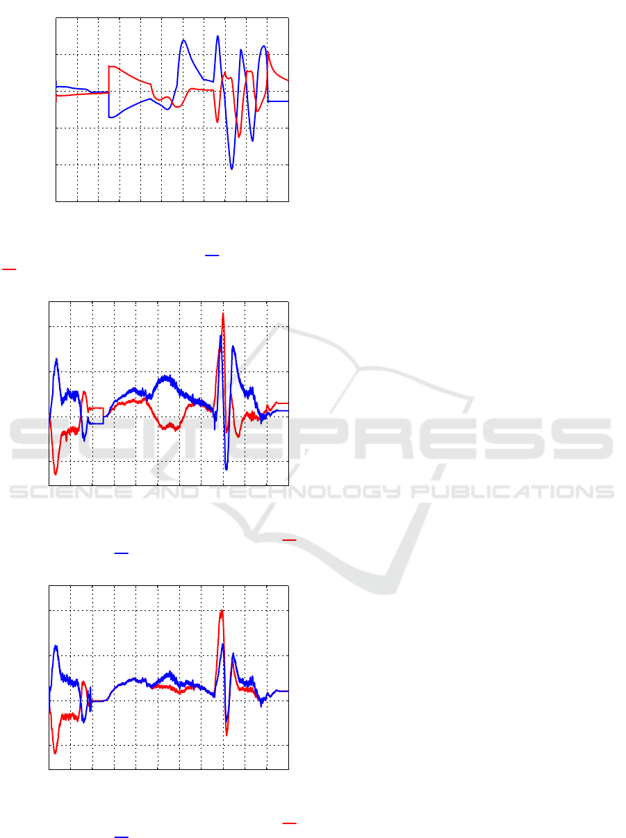
t in s

0 2 4 6 8 10 12 14 16 18 20 22

−1.5

−1

−0.5

0.5

s1d

− ϕ

◦

Figure 6: Steering tracking error for the classic PD and

replacements

model-based controlled front wheel i = 1.

τ in Nm

t in s

0 2 4 6 8 10 12 14 16 18 20

−5

Figure 7: Driving torque for the classic DP control.

Front wheel i = 1 and rear wheel i = 2.

τ in Nm

t in s

0 2 4 6 8 10 12 14 16 18 20 22

−5

Figure 8: Driving torque for the model-based control.

Front wheel i = 1 and rear wheel i = 2.

6 SUMMARY AND OUTLOOK

In this work a model-based dynamic control con-

cept is introduced for redundantly actuated, non-

holonomic and omnidirectional vehicles with n cen-

tered orientable standard wheels.

The ﬁrst part of this paper introduces a framework

for the dynamic modeling of such vehicles, including

friction and inertia effects. It turned out, that the kine-

matic constraints of the vehicle are permanently sin-

gular or can become singular. Therefore the dynam-

ics is modeled with a redundant set of coordinates.

This formulation does not eliminate unknown trac-

tion forces (constraint forces) in the dynamic equa-

tions but is in each conﬁguration, especially in singu-

lar conﬁgurations, valid. The elimination of the con-

straint forces is done through projecting the dynamics

equation with a null space projector of the constraints.

This projector is computed in a highly efﬁcient man-

ner by a semi-analytical approach.

The second part uses this model for an augmented

PD-control consisting of an inverse dynamics compo-

nent as well as a stabilizing feedback PD control law.

The distribution of the computed torque among the

different actuators is done through a weighted least

square approach. Whereby wheels with a higher stall

torque, which is the maximum motor torque that does

not result in slippage, during accelerating the chassis

against a mechanical stop, are less weighted. A PD

control is additionally used to asymptotically stabilize

the vehicle along a desired motion. The counteraction

is thereby avoided by using the projected velocity er-

ror instead of the individual wheel velocity errors.

Future work will focus on the online identiﬁcation

of the load weight and the frictional conditions. This

knowledge can be used to adapt the parameters of the

inverse dynamics as well as the torque balancing law

which improves the robustness of the concept. Ad-

ditionally, the dynamic model will be used to moni-

tor the vehicles state enabling a higher-level logic to

detect faults on the drive units and unexpected colli-

sions.

ACKNOWLEDGEMENTS

This work has been supported by the Austrian

COMET-K2 program of the Linz Center of Mecha-

tronics (LCM), and was funded by the Austrian fed-

eral government and the federal state of Upper Aus-

tria.

Dynamic Model-based Control of Redundantly Actuated, Non-holonomnic, Omnidirectional Vehicles

REFERENCES

Bj¨orck,

A. (1994). Numerics of gram-schmidt orthog-

onalization. Linear Algebra and Its Applications,

197:297–316.

Bona, B. and Indri, M. (2005). Friction compensation in

robotics: an overview. In Conference on Decision

and Control and European Control Conference, pages

4360–4367. IEEE.

Campion, G., Bastin, G., and D’Andr´ea-Novel, B. (1996).

Structural properties and classiﬁcation of kinematic

and dynamic models of wheeled mobile robots. Trans-

actions on Robotics and Automation, 12:47–62.

De Luca, A., Oriolo, G., and Samson, C. (1998). Feed-

back control of a nonholonomic car-like robot. In

Robot motion planning and control, pages 171–253.

Springer.

Fukao, T., Nakagawa, H., and Adachi, N. (2000). Adap-

tive tracking control of a nonholonomic mobile robot.

Robotics and Automation, IEEE Transactions on,

16(5):609–615.

Giordano, P. R., Fuchs, M., Albu-Sch¨affer, A., and

Hirzinger, G. (2009). On the kinematic modeling and

control of a mobile platform equipped with steering

wheels and movable legs. In International Confer-

ence on Robotics and Automation, pages 4080–4087.

IEEE.

Hall, D. E. and Moreland, J. C. (2001). Fundamentals of

rolling resistance. Rubber chemistry and technology,

74(3):525–539.

Lee, M.-H. and Li, T.-H. S. (2015). Kinematics, dynamics

and control design of 4wis4wid mobile robots. In The

Journal of Engineering, volume 1. IET.

M¨uller, A. (2011). A robust inverse dynamics formula-

tion for redundantly actuated pkm. In 13th World

Congress in Mechanism and Machine Science, Gua-

najuato, Mexico, pages 19–25.

M¨uller, A. and Hufnagel, T. (2012). Model-based control of

redundantly actuated parallel manipulators in redun-

dant coordinates. Robotics and Autonomous Systems,

60(4):563–571.

Murray, R. M., Li, Z., Sastry, S. S., and Sastry, S. S. (1994).

A mathematical introduction to robotic manipulation.

CRC press.

Oftadeh, R., Ghabcheloo, R., and Mattila, J. (2013). A

novel time optimal path following controller with

bounded velocities for mobile robots with indepen-

dently steerable wheels. In International Conference

on Intelligent Robots and Systems, pages 4845–4851.

IEEE.

Ostrowski, J. and Burdick, J. (1996). Geometric perspec-

tives on the mechanics and control of robotic locomo-

tion. In Robotics Research, pages 536–547. Springer.

Ploeg, J., van der Knaap, A. C., Verburg, D. J., and Auto-

motive, T. (2002). Design, implementation and evalu-

ation of a high performance agv. In Intelligent Vehicle

Symposium. IEEE.

St¨oger, C., M¨uller, A., and Gattringer, H. (2015). Kine-

matic analysis and singularity robust path control of a

non-holonomic mobile platform with several steerable

driving wheels. In International Conference on Intel-

ligent Robots and Systems, pages 4140–4145. IEEE.

Yang, J.-M. and Kim, J.-H. (1999). Sliding mode control for

trajectory tracking of nonholonomic wheeled mobile

robots. Robotics and Automation, IEEE Transactions

on, 15(3):578–587.

ICINCO 2016 - 13th International Conference on Informatics in Control, Automation and Robotics