Electric Power System Operation: A Petri Net Approach for Modeling
and Control
Milton Souza
1
, Evangivaldo Lima
2
and J´es Cerqueira
3
1
Faculdade de Tecnologia Senai-Cimatec, Avenida Orlando Gomes, Piat˜a, Salvador, Bahia, Brazil
2
Universidade do Estado da Bahia, Rua Silveira Martins, Salvador, Bahia, Brazil
3
Universidade Federal da Bahia, Aristides Novis, Salvador, Bahia, Brazil
Keywords:
Petri Nets, Electric Power System, Model, Supervisor, Constraint.
Abstract:
In this paper the operation of electric power system is treated as a discrete event system and a Petri Net is
used as formal tool to achieve it. Each component of power system is modelled as a single Petri Net and the
complete model is reached by composition of these single Petri Nets. Properties such as: parallelism, conflict,
concurrency and others are used to study the operation of the modelled system. In this study are detected
undesired behaviors on the dynamics of system. The theory of supervisory control is used to avoid these
undesired behaviors forcing the system to have a controlled behavior. To obtain a controlled system a set of
constraint are modelled by linear inequalities and the systems is forced to obey it. A case study application is
presented to illustrate the proposed model here.
1 INTRODUCTION
The power system is modeled using math tools such
as, differential equations and the main goal is to ob-
tain the optimal operation state. In the basic level, the
power system generates, transforms and distributes
the electric power to the loads.
Next, there is the layer of control equipment. This
equipment helps maintain the power system at its nor-
mal voltage and frequency, generates sufficient power
to meet the load and maintains optimum economy and
security in the interconnected network. The control
equipment is organized in a hierarchy of its own, con-
sisting of local and central control functions.
The equipments control of electric power systems
is governed by a set of procedures that are required
to ensure that any intervention on the system and will
be performed under safe condition, considering the
inherent dangers coming from the presence of live
conductors, parts and components. In the last years
the formalization of the general rules and methods
adopted in the preparation, control and actuation of
electrical procedures has been proposed. The Electric
Power System modeling using Petri nets is one of this
formal methods used by researchers.
In this sense, the system evolution and its state
changes is obtained in graphical and analytical form
allowing the better understand of logic in the proce-
dures and to allow its immediate consistency. In ad-
dition, the check of the correctness of the procedures’
operating sequences could be followed. In the work
of (A. Ashouri and Noroozian, 2010), the Petri nets is
used, in addition of SCADA system, to diagnose fault
protection elements. In (Vescio et al., 2015) has been
used Marked Petri nets to represent EPS and through
its dynamics and mathematical structure to find unde-
sirable conditions. In this work is presented the equip-
ment control of electric power systems using supervi-
sory control theory and Place Invariants of Petri nets
(Lima and D´orea, 2002).
In this sense, this paper is organized as follow:
In the section 2 is presented the theoretical basis of
supervisory control using place invariants of Petri
Nets(PN). Electric Power Systems(EPS) is described
in the section 3. The case study is treated in the sec-
tion 4. Conclusions and future expectations end this
work.
2 SUPERVISORY CONTROL
Many researchers used Petri nets as a tool for model-
ing, analyzing and synthesize control laws for DES.
There are many works applied in the literature (Mu-
rata, 1989),(Boissel and Kantor, 1995),(Zhou and
Souza, M., Lima, E. and Cerqueira, J.
Electric Power System Operation: A Petri Net Approach for Modeling and Control.
DOI: 10.5220/0005977904770483
In Proceedings of the 13th International Conference on Informatics in Control, Automation and Robotics (ICINCO 2016) - Volume 1, pages 477-483
ISBN: 978-989-758-198-4
Copyright
c
 2016 by SCITEPRESS – Science and Technology Publications, Lda. All rights reserved
477

Dicesare, 1992),(Boucher, 1996), (Moody, 1998).
Assuming the model of a given modeled plant
in Rdp is (N, M
0
) where N = (P, T, D, W) and D =
Post − Pre is a set of all reachable markings starting
in the initial mark M
0
in the corresponding PN. As-
suming also that the control objective is to restrict the
state plant evolution from state S to subset S
′
, S
′
∈ S.
This constraint imposed by the control is described by
a set of linear inequalities:
L∗ M(k) ≤ b (1)
Where L ∈ Z
qxn
, b ∈ Z
q
, M ∈ Z
m
.
The compured controller will act not only to allow
the firing for a transition leading to the occurrence of
an unwanted state. It sets an extreme condition of the
controller action. To determine the unknown param-
eters of the controller: M
c
(0) e D
c
is calculated as
follows:
From the control specifications given in equation 1 is
noted that
L∗ M(k) + M
c
(k) = b, (2)
where k = 0, 1, . . . m and M
c
(k) is a positive vector of
integers inserted as a break to make the inequality in
equality. For k = 0 is determined that the driver mark
is given by:
M
c
(0) = b− L∗ M(0) (3)
2 - Multiplying both sides of equation 5 by the ma-
trix [L I] and applying invariance property from the
equation 2, it is determined that the controller inci-
dence matrix is given by:
D
c
= −L∗ D (4)
The equations 3 and 4 are used for solve control
problems. The equation 3 is used to compute initial
marking to the controller while equation 4 show how
Places-controller are linked with transitions in the
plant(EPS model) (Lima and D´orea, 2002), (Moody,
1998).
The controllers are places linked by arcs in the
model pc
1
, . . . , pc
q
and their marking M
c
(k) ∈ N
q
re-
spectively. The initial marking and the way the con-
troller is connected to transitions can be obtained by
taking an extended Petri net with (M, M
c
)
T
. If a tran-
sition t
j
fire,the PN state change according the equa-
tion 5.

M(k+ 1)
M
c
(k+ 1)

=

M(k)
M
c
(k)

+

D
D
c

∗ σ
j
(5)
3 ELECTRIC POWER SYSTEM
The Electric Power Systems can be defined as a set
of physical equipment and connected electrical circuit
elements, which act in a coordinated manner in order
to generate, transmit and distribute electrical energy
to consumers. The generation makes up the func-
tion of converting some form of energy into electri-
cal, transmission carries electricity from production
centers to consumption centers or to other electrical
systems, connecting them. Distribution distributes the
power received from the transmission system to large,
medium and small consumers (Vescio et al., 2015).
3.1 Modeling of Electric Power Systems
(EPS)
The electrical system should be carefully represented
by appropriate modeling tool. The tool has relation-
ship to type of study to be performed. For protec-
tion studies, for example, values of short-circuit cur-
rents should be calculated. Therefore, each system
component must be modeled and represented from
the perspective of its behavior to short-circuit cur-
rents. This modeling is relatively easy due to the
simplifications made in the equivalent circuits of the
components. The suitability of the model for stud-
ies of short-circuit is made with the use of symmetri-
cal components, which leads to the obtaining of three
system models: positive sequence, negative sequence
and zero sequence (Grainger and Stevenson, 1994).
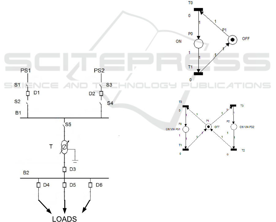
3.2 Single Line Diagram of EPS
Because the system operates normally balanced, it
replaces its three-phase representation by a sym-
bolic representation, known as single-line diagram.
The importance of the single-line diagram is clearly
present the topology and concisely the significant
power system data. The single-line diagram can con-
tain different information depending on the type of
study, such as for power flow, short circuit, stabil-
ity and protection (Anderson, 1998). An example of
single-line diagram is shown in Figure 1.
3.3 Elements of Electric Power System
The electric power systems can be composed of some
basic components that together have the function gen-
erate, transmit, distribute or connect other electrical
power systems (Grainger and Stevenson, 1994). some
of these elements are:
1. Generator - Element active power generator
2. Power Transformer - They increase or decrease
the currents and voltages of the EPS
3. Transformer as Mesure Instrument - parame-
ters in order to monitor, control and protection.
ICINCO 2016 - 13th International Conference on Informatics in Control, Automation and Robotics
478

4. Bus - elements used as points of interconnection
between the EPS components.
5. Breakers - Switching used to turn on or off a EPS
normal or abnormal condition.
6. Switch - Device designed to isolate (sectioning)
parts (subsystems, equipment etc.) of electrical
circuits. They are installed aiming at breaking the
network to minimize the effects of planned out-
ages or not, establish visible sectioning in equip-
ment such as automatic circuit reclosers, switches
oil, establish bypass in equipment such as voltage
regulators, etc.(Grainger and Stevenson, 1994).
4 MODELING OF EPS
OPERATION USING
PLACE-TRANSITION PETRI
NETS
This chapter is a case study of modeling a EPS us-
ing Place-Transition Petri net. Therefore, it has to be
a single line diagram EPS consisting of 2 buses (B
1
and B
2
) 6 circuit breakers (D
1
, D
2
,· · · ,D
6
), 5 switches
(S
1
,· · · , S
5
) 1 transformer and 3 energy consumers.
Figure 1 shows the single line diagram for this study.
Figure 1: Bus Feeder System and Power Supply.
From:(ABB, 2010).
4.1 Modeling of the EPS Free Behavior
The development of the free behavior model in PN as-
sociated to elements of the EPS Figure 1, taking into
account:
• breakers and switches have two possible states on
or off
• The transformer T and buses B
1
and B
2
will be
modeled by three states, which are power off state,
energized via feeder PS
1
and energized via feeder
PS
2
• In this model will not be provided abnormal oper-
ation of the elements.
The Figures 2 and 3 show these representations in
Petri net. The presence of token in a place will in-
dicate the current state of the element.
Figure 2: Petri Net Model for Switch and Breaker.
Figure 3: Petri Net Model For Transformer and Bus.
From the individual model, determines the com-
plete model of the system. The composition of PS
1
feeder is shown in Figure 4. The places of P
1
to P
6
represent the sets of circuit breaker and switches that
will energize the input bus B
1
, P
7
represents that Bus
B
1
is energized via PS
1
and P
8
the opposite state. the
complete model is made by 6 places representing PS
2
P
9
to P
13
. The same way bus B
1
, the transformer and
the output bus B
2
have in their models information
about power supply origin see Figure 3. They have
three places those represent energized via PS
1
or PS
2
and another to represent the off-state. The transformer
Electric Power System Operation: A Petri Net Approach for Modeling and Control
479

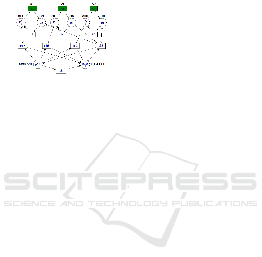
Figure 4: Model of Free Behavior of the EPS.
is represented by the states P
19
, P
20
and P
21
and the
output bus B
2
by the states P
24
, P
25
and P
26
respec-
tively. Power up these elements are linked to S
5
and
D
3
when P
18
and P
23
are marked. All consumers are
powered up by individual circuit breakers represented
by places P
27
to P
32
that enable energy consumption
by two distinct paths PS
1
and PS
2
. To represent con-
sumers, the model has places of infinite capacity with
dual transition. The enabled transitions provide infor-
mation about the origin of the supplied energy. The
even transitions are enabled and fired when the power
supply is PS
1
and odd transitions PS
2
.
4.2 Supervisory Control Theory
Applied to EPS
The free behavior of the proposed example presents
several EPS operating problems. There are charac-
teristics of power components that make up a EPS to
be taken into account when turn on or off the power.
As shown in (Zhao and Mi, 2006) breakers are the
EPS equipment designed to make power on and off.
Switches should isolate or integrate a region of a EPS
when in power off state.
To avoid the modeled example may have improper
representation (eg open switch when circuit breaker is
on state) should expand this PN model putting super-
visors places distributed in all sectors of the prior PN.
These places are dedicated to develop constraints in
breakers and switches models as shown in (Zhao and
Mi, 2006). The following constraints are identified in
the studied model:
1. The procedures for energization via B
1
must start
with the connection of the keys S
1
and S
2
. For
this, you should impose the following constraint,
M
P
2
+ M
P
6
≤ 2;
2. After the P
36
controller close the switches S
1
and
S
2
, the circuit breaker controller of D
1
receives
the privilege for its opening or closing, 2∗ M
P
4
+
M
P
36
≤ 2;
3. Similarly, energization via B
2
must start with the
connection of the keys S
3
and S
4
. For this, you
should impose the following constraint, M
P
9
+
M
P
13
≤ 2;
4. After the controller P
38
close the switches S
3
and
S
4
, the circuit breaker controller of D
2
should gain
the status to take any action on it. this restriction
is described as follows: 2∗ M
P
11
+ M
P
38
≤ 2;
5. The switch S
5
may change status (on / off) when
the input bus is power off. This is possible to cre-
ate a Constraint from the state that is power the
bus off P
16
and the state is S
5
connected P
18
then
we have: M
P
16
+ M
P
18
≤ 1;
6. The controller for handling breaker D
3
of the out-
put bus energization will have autonomy to op-
erate it only when the status of switch S
5
is on.
This condition generates inequality linked with
the marking of the states that represent them, P
17
and P
22
. It is then: M
P
17
+ M
P
22
≤ 1;
7. The last supervisor shall be responsible for rout-
ing the way which will be energized when the bus
power down. The supervisor function is monitor
the B
1
power down through the place (P
16
. It is
write the following restriction:. M
P
16
+ M
P
7
≤ 1
To illustrate the implementation of the controllers
consider the inequalities generated from the feeder
free behavior modelPS
1
. As shown in the literature,
see (Grainger and Stevenson, 1994), the maneuvers of
switches and circuit breakers must comply their con-
structive features as real representative system. Thus,
the model dynamic should express such conditions.
So supervisor control theory will restrict the model
dynamics. The new PN transform the free behavior
in the actual operating conditions of EPS elements.
From item 1 and 2 above, follow the equations:
a) Constraint M
P
2
+ M
P
6
≤ 2

0 1 0 0 0 1

∗







M
P
1
M
P
2
M
P
3
M
P
4
M
P
5
M
P
6







≤ [2]
b) Constraint 2∗ M
P
4
+ M
P
36
≤ 2

0 0 0 2 0 0 1

∗









M
P
1
M
P
2
M
P
3
M
P
4
M
P
5
M
P
6
M
P
36









≤ [2]
Extracting the PNs for both cases the incidence matri-
ces and the initial marking (D
1
and M
10
) and (D
2
and
ICINCO 2016 - 13th International Conference on Informatics in Control, Automation and Robotics
480

M
20
) we have:
D
1
=







−1 1 0 0 0 0
1 −1 0 0 0 0
0 0 −1 1 0 0
0 0 1 −1 0 0
0 0 0 0 1 −1
0 0 0 0 −1 1







e M
01
=

1 0 1 0 1 0

T
D
2
=









−1 1 0 0 0 0
1 −1 0 0 0 0
0 0 −1 1 0 0
0 0 1 −1 0 0
0 0 0 0 1 −1
0 0 0 0 −1 1
−1 1 0 0 −1 1









e M
02
=

1 0 1 0 1 0 2

T
by these information and using equations3 and 4 are
found the controller 1 and 2 characteristics. Such in-
formation are represented in the expanded Petri net by
places P
36
and P
37
;
a) controller1 Features
D
c1
=

−1 1 0 0 −1 1

M
c10
= [2]
b) Controller2 Features
D
c2
=

1 −1 2 −2 1 −1

M
c20
= [0]
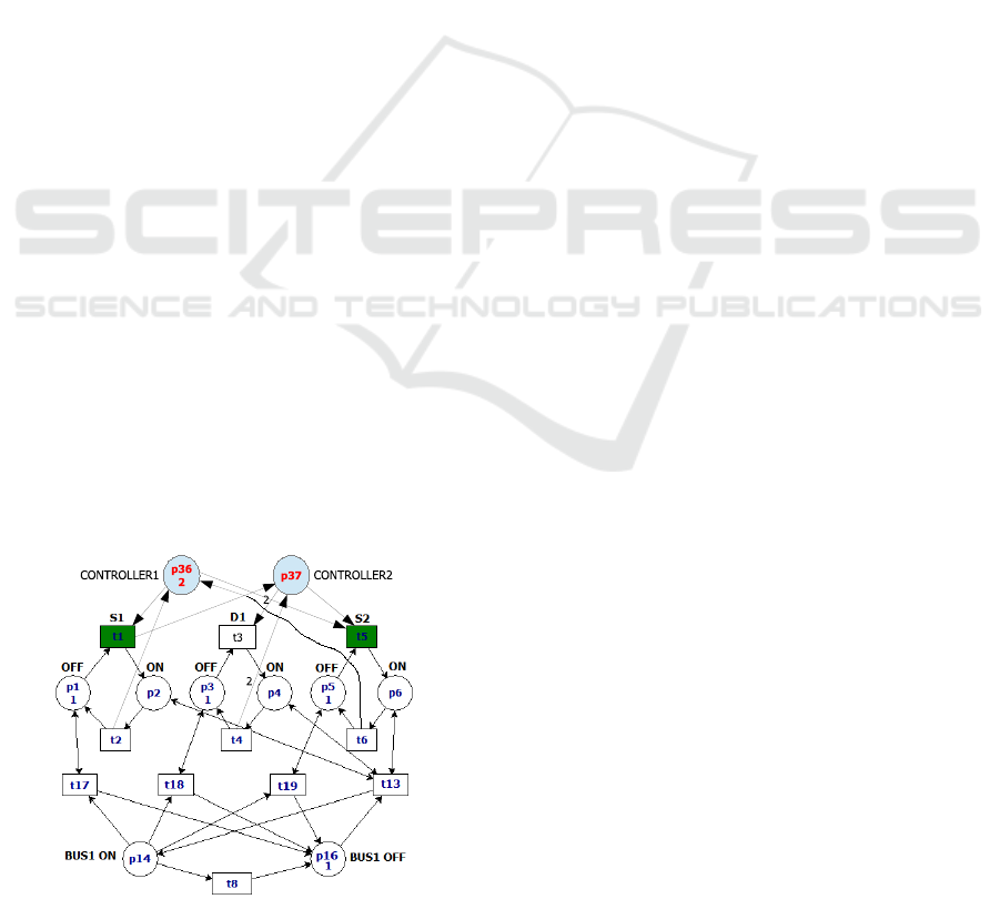
Figure 5 shows the expanded model of Petri net feeder
(PS
1
) bus of the EPS case study. The Figure 5 shows
that the PN is started with switches and Breaker in off
state (P
1
, P
3
and P
5
with marking). In this condition,
only Controller1 is enabled (P
36
2 marks) allowing the
switches models S
1
and S
2
go to the on state. t
1
and
Figure 5: Petri Model of PS
1
Feeder.
t
5
firing takes P
2
and P
6
to receive tokens represent-
ing the switches were turned on. This sequence of
firing takes disabling Controller1 and enabling Con-
troller2 that received 2 marks. This condition enables
the transition t
3
firing takes the model of D
1
to on
state, meaning that B
1
was energized. The same con-
dition can be obtained by the equation 5











M
1
M
2
M
3
M
4
M
5
M
6
M
c
1
M
c
2











=











1
0
1
0
1
0
2
0











+


D
D
c
1
D
c
2


∗ σ (6)
Where


D
D
c
1
D
c
2


=











−1 1 0 0 0 0
1 −1 0 0 0 0
0 0 −1 1 0 0
0 0 1 −1 0 0
0 0 0 0 −1 1
0 0 0 0 1 −1
−1 1 0 0 −1 1
1 −1 −2 2 1 −1











and σ is the transition sequence that will fire, t
1
t
3
t
5
σ =

1 0 1 0 1 0

T
computing get the following result:

0 1 0 1 0 1 0 0

T
The result shows the PN conditions obtained in pre-
vious analysis. Places P
2
, P
4
and P
6
receive marks
representing the circuit breaker and switches in on
states. This condition makes the transition t
13
en-
abled, if fire, place P
16
loss marking (Bus Off) to
place P
14
(Bus On) indicating bus B
1
power on via
PS
1
. Note that transition t
13
is connected to places
by self-loops. this connection maintain narking after
t
13
firing. This is critical to guarantee the states of
switches and breakers with bus power on. The Figure
6 is a simplified way to represent EPS PN model stud-
ied with controllers those restrict the free behavior of
their switches and circuit breakers. The figure shows
two-way arrows to show the flow of PN-controller in-
formation. Thus, if transition t
j
fires, the controller
receives or losses marking given by the weight of its
arcs. The set of controllers C
1
, C
2
, C
3
, C
4
, C
5
and C
6
receive information through their enabled input tran-
sitions or disable other output transition. these actions
impose free behavior model(without control) com-
ply the constraints those are imposed. Such dynamic
avoid firing transitions those take the PN to forbidden
Electric Power System Operation: A Petri Net Approach for Modeling and Control
481

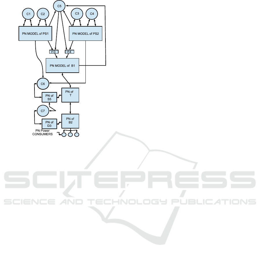
Figure 6: Simplified diagram of the PN Expanded with con-
trollers.
state. opening of the switch S
1
with the breaker D
1
closed is a forbidden state.
Note the Figure 6 that set of controllers C
1
and
C
2
, C
3
and C
4
are controllers of the PN feeders PS
1
and PS
2
. The controller C
5
selects the path that the
expanded PN will represent B
1
state energized or via
PS
1
or via PS
2
. These dynamics two ways for take B
1
in on state:
• P
14
which indicates that model is energizing via
PS
1
;
• while the state P
15
represent energizing via PS
2
.
To energize the transformer, the EPS example, uses
the switch S
5
. S
5
operation should be done when
the bus is power off and the secondary of the trans-
former devoid of energy consumers. Thus, the repre-
sentative model of the EPS should include such re-
strictions. The constraints have been implemented
through two controllers C
6
and C
7
. C
6
function is re-
stricting against closing S
5
for energized bus andC
7
is
restricting against opening with circuit breaker D
3
in
on state. C
6
and C
7
are represented in simplified PN
block diagram Figure 6.
5 CONCLUSION
The electric power system operation is completely
modeled by a Petri nets. The model can be achieved
through the creation of single PN for each part of sys-
tem. The free behavior of each elements that make up
the system then are interconnected to form the repre-
sentation of power system. This representation is free
of any constraint of the elements make up the EPS.
This article was called free model or free behavior of
the electric power system.
The existing memory effect on the opening and
closing of a circuit breaker in the PN model was
solved using a feature of Petri nets called self-loop.
This is done by interconnecting one place and transi-
tion by two arcs in opposite directions to each other.
Thus, the turn on circuit breaker do not lost a token
by energizing a bus transition is enabled by the place
up switch can shoot without any loss of the marking
place in dynamic network.
The model of free behavior of the electric power
system does not describe the actual behavior of EPS
elements. Decoupling between individualized mod-
els of its elements provide the appearance of undesir-
able states or states that would cause risk to integrity
of the EPS. To eliminate such states, the model was
expanded using local supervisors. The Local super-
visors are places inserted in the free model that have
the ability to restrict undesirable states through inhi-
bition of controllable transitions firing. The imple-
mentation of these controllers are made from inequal-
ities that describe such constraint. These inequations
determining the initial marking, the weights of input
and output arcs for each supervisor. The evolution of
the dynamics of the new network is presented as a se-
quence of markings of places that fully comply with
the procedures and or care that you have to turn on or
off an electric power system without weakening the
actual functionality of the EPS.
The existing mememory effect on the opening and
closing of a switcher and breaker in the PN model
was solved using a feature of Petri nets called self-
loop. This is done by interconnecting one place and
transition by two arcs in opposite directions to each
other. Thus, the turn on switcher do not lost a token
by energizing a bus transition is enabled by the place
up switch can shoot without any loss of the marking
place in dynamic network.
The model of free behavior of the electric power
system does not describe the actual behavior of EPS
elements. Decoupling between individualized mod-
els of its elements provide the appearance of undesir-
able states or states that would cause risk to integrity
of the EPS. To eliminate such states, the model was
expanded using local supervisors. The Local super-
visors are places inserted in the free model that have
the ability to restrict undesirable states through inhi-
bition of controllable transitions firing. The imple-
mentation of these controllers are made from inequal-
ities that describe such constraint. These inequations
ICINCO 2016 - 13th International Conference on Informatics in Control, Automation and Robotics
482

determining the initial marking, the weights of input
and output arcs for each supervisor. The evolution of
the dynamics of the new network is presented as a se-
quence of markings of places that fully comply with
the procedures and or care that you have to turn on or
off an electric power system without weakening the
actual functionality of the EPS.
Going beyond that as future work should improve
the model by entering the protection elements and ap-
ply this model in the study of diagnosability.
REFERENCES
A. Ashouri, A. J. and Noroozian, R. (2010). Fault diagnosis
modeling of power systems using petri nets. pages
23–24. IEEE.
ABB (2010). Abb special report iec 61850. Technical re-
port.
Anderson, P. M. (1998). Analysis of faulted power systems.
Boissel, O. R. and Kantor, J. C. (1995). Optmal feedback
control design for discrete event systems using sim-
ulated annealing. Elsevier Science LTD, 19(3):253–
266.
Boucher, T. O. (1996). Computer Manufacturing and Au-
tomation.
Grainger, J. and Stevenson, W. D. (1994). Power System
Analysis.
Lima, E. A. and D´orea, C. E. T. (2002). An algorithm for
supervisory control of discrete event system via places
invariants. In IFAC.
Moody, J. O. (1998). Supervisory Control of Dicrete Event
System Using Petri Nets.
Murata, T. (1989). Petri nets: Properties, analysis and ap-
plications. volume 77, pages 541–580. Proceedings of
IEEE.
Vescio, G., Riccobon, P., Grasselli, U., and Angelis, F. D.
(2015). A petri net model for electrical power systems
operating procedures. In Reliability and Maintainabil-
ity Symposium (RAMS), 2015 Annual, pages 1–6.
Zhao, H. and Mi, Z. (2006). Modeling and analysis of
power systems events. In IEEE.
Zhou, M. C. and Dicesare, F. (1992). Design and imple-
mentation of a petri net based supervisor for a flexi-
ble manufacturing system. International Federation
of Automatic Control, 28(6).
Electric Power System Operation: A Petri Net Approach for Modeling and Control
483