Autoencoder Networks for Water Demand Predictive Modelling

Ishmael S. Msiza and Tshilidzi Marwala

Faculty of Engineering & The Built Environment, University of Johannesburg, Auckland Park, Johannesburg, South Africa

Keywords:

Neural Network, Autoencoder Network, Multi-layer Perceptron, Water Demand, Time Series, Regression

Approximation, Predictive Modelling, Hidden Units, Network Dimensionality, Arbitrary Complexity.

Abstract:

Following a number of studies that have interrogated the usability of an autoencoder neural network in various

classiﬁcation and regression approximation problems, this manuscript focuses on its usability in water demand

predictive modelling, with the Gauteng Province of the Republic of South Africa being chosen as a case study.

Water demand predictive modelling is a regression approximation problem. This autoencoder network is

constructed from a simple multi-layer network, with a total of 6 parameters in both the input and output

units, and 5 nodes in the hidden unit. These 6 parameters include a ﬁgure that represents population size

and water demand values of 5 consecutive days. The water demand value of the ﬁfth day is the variable of

interest, that is, the variable that is being predicted. The optimum number of nodes in the hidden unit is

determined through the use of a simple, less computationally expensive technique. The performance of this

network is measured against prediction accuracy, average prediction error, and the time it takes the network

to generate a single output. The dimensionality of the network is also taken into consideration. In order to

benchmark the performance of this autoencoder network, a conventional neural network is also implemented

and evaluated using the same measures of performance. The conventional network is slightly outperformed

by the autoencoder network.

1 INTRODUCTION

Artiﬁcial neural networks – simply known as neural

networks – occur in many different forms and types,

and one of these types is known as an autoencoder

network. This is a network trained to recall its in-

put, and the purpose of the work presented in this

manuscript is to interrogate the usability of this net-

work in a predictive modelling application. This ap-

plication involves the analysis and prediction of a wa-

ter demand time series. This interrogation is informed

by the constantly eminent need that neural network

practitioners have to, whenever possible, reduce the

dimensionality or size of any neural network. An au-

toencoder network is known for its ability to compress

data (Marivate et al., 2008), hence it is chosen for the

dimensionality reduction component of this study.

The importance of having a neural network with

reduced dimensionality is presented as part of the the-

ory of autoencoder networks in section 2. The state

of the current literature – regarding autoencoder net-

work applications – is presented in section 3, and the

implementation of this network in water demand pre-

dictive modelling – together with the evaluation of its

performance – is discussed in section 4. In order to

endorse the performance of this autoencoder network,

it is necessary or useful to compare it against that of

a conventional neural network. The implementation

of this conventional network is presented in section 5,

and the comparison between the two models is car-

ried out in section 6, just before the conclusions and

proposed future work in section 7.

2 NEURAL NETWORKS

This section of the manuscript serves to introduce the

theory of conventional neural networks, in general,

and autoencoder neural networks, in particular.

2.1 Conventional Neural Networks

A neural network could be deﬁned as a computer-

based machine that is designed to model the way in

which the human brain executes a particular task or

function of interest (Marwala, 2016). What this im-

plies is that, a neural network is a computer model

that is taught to duplicate the manner in which the

human brain performs a given task. Because the op-

Msiza, I. and Marwala, T.

Autoencoder Networks for Water Demand Predictive Modelling.

DOI: 10.5220/0005977202310238

In Proceedings of the 6th International Conference on Simulation and Modeling Methodologies, Technologies and Applications (SIMULTECH 2016), pages 231-238

ISBN: 978-989-758-199-1

231

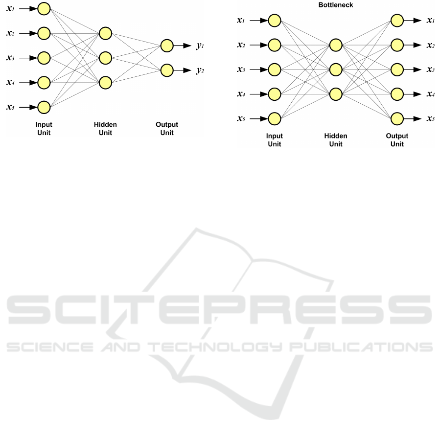
Figure 1: An example of a simple MLP neural network that

has 2 layers of weighted connections and 3 layers of pro-

cessing units.

erations of the brain are primarily facilitated by struc-

tures known as biological neural networks (van De-

venter and Mojapelo-Batka, 2013), a computer-based

neural network is speciﬁcally referred to as an artiﬁ-

cial neural network.

When sketched on a piece of paper, a neural net-

work looks like a physical linkage of processing units

through weighted connections. It can occur in the

form of various architectures, including a multi-layer

perceptron (MLP) and a radial basis function (RBF).

The MLP is, however, the most common neural net-

work architecture in terms of use. It is important to

note that an MLP network can be conﬁgured in the

form of any number of weighted connections, but

many practitioners have demonstrated that a neural

network conﬁgured to have two weighted connections

is capable of modelling just about any functional map-

ping, however complex it may be. This is a network

with three processing units: the input unit, the hidden

unit, and the output unit. Figure 1 depicts an example

of a simple MLP network that has ﬁve inputs, three

hidden nodes, and two outputs.

2.2 Autoencoder Neural Networks

An autoencoder network is a type of the conventional

neural network. For the conventional neural network

to be regarded as an autoencoder neural network, it

has to conform to the following two rules.

• Autoencoder Rule 1: the neural network has to

be auto-associative.

• Autoencoder Rule 2: the hidden unit of the net-

work has to be narrow, that is, the network must

have what is often referred to as a bottleneck.

Its auto-associative nature implies that the autoen-

coder network tries to associate the input unit with

the output unit, so as to minimize the error between

the two. In practical terms, this implies that – when

Figure 2: An example of an autoencoder neural network. It

has 5 inputs, 3 nodes in the hidden unit, and 5 outputs.

presented with a set of inputs – the autoencoder net-

work attempts to produce the same set of inputs in the

output unit. The immediate advantage of this behav-

ior is that this network can map both the linear and the

non-linear relations between all the inputs (Thompson

et al., 2002).

The bottleneck implies that the number of nodes

in the hidden unit should be less than the number of

nodes in both the input and output units. This results

in a network that has a narrow hidden unit, with the in-

put and output units having the same size, hence hav-

ing a butterﬂy-like structure, as depicted in ﬁgure 2.

This bottleneck compresses the input space data into a

smaller dimension, then decompresses it into the out-

put space. The key advantage of having a narrow hid-

den unit is that the network becomes less complex,

and its dimensionality (size) is reduced. This is be-

cause of the fact that the complexity of a neural net-

work has a directly proportional relationship with the

number of nodes in the hidden unit.

The number of nodes in the hidden unit is also pro-

portional to the dimensionality of the network. A net-

work with large dimensionality tends to have a small

error between the input and output data during the

training process, but this error increases when the net-

work is presented with previously unseen data. A net-

work that behaves in this manner is said to have poor

generalization ability. This, therefore, implies that the

idea behind using an autoencoder network is to have

a system that: has low dimensionality, is less com-

plex, is accurate, and has good generalization abil-

ity. These factors play an important role in the per-

formance evaluation of a predictive modelling system

that is based on neural computing.

2.3 Optimum Dimensionality Selection

When using neural networks (conventional or other-

wise), one of the most important exercises is the pro-

SIMULTECH 2016 - 6th International Conference on Simulation and Modeling Methodologies, Technologies and Applications

232

cess of selecting the optimum number of nodes in the

hidden unit, that is, the optimum dimensionality of

the network at hand. This exercise is a form of model

tuning and optimisation. Just to demonstrate how im-

portant this exercise is, some pratitioners dedicate an

entire document writing about model tuning and opti-

misation (Hessel et al., 2014). When dealing with an

autoencoder network, this exercise becomes less un-

certain because – when taking Autoencoder Rule 2,

mentioned above, into consideration – the following

condition will always be true:

1 ≤ N

hidden

≤ (M −1), f or M = N

input

= N

out put

(1)

where N

hidden

is the number of nodes in the hidden

unit, M is a value that is equal to the number of nodes

in both the input and output units, N

input

and N

out put

Equation 1 implies that the optimum number of nodes

in the hidden unit will be a value that is between 1 and

(M − 1).

In order to select this optimum number of nodes

in the hidden unit, this work takes advantage of cross-

validation and introduces a variable called ∆E. Cross-

validation is a technique used to monitor and evalu-

ate the network’s performance, where the dataset in-

volved is split into three partitions: the training set,

the validation set, and the testing set. For the com-

plexity of this study, a single round of cross-validation

is sufﬁcient. For more complex studies, it is often

necessary to perform multiple rounds, while rotating

these partitions of data. ∆E is a measure of the change

in average error between the training and validation

data sets. It is an indication of the trained model’s

generalization ability. It is mathematically deﬁned

as the arithmetic difference between the average er-

ror obtained from the training data set – the average

training error, E

training

– and the one from the valida-

tion data set – the average validation error, E

validation

– as indicated in equation 2.

∆E = E

training

− E

validation

(2)

Because this measure only uses the training and the

validation data sets, it could be said that it uses the

hold-out (train and test) method, which is the sim-

plest form of the cross-validation technique. Using

this measure to select the optimum number of nodes

in the hidden unit, it is essential to heed these three

important notes:

• Note A: this change in error can have a positive

or a negative value.

• Note B: a negative value indicates that the number

of nodes in the hidden unit leads to poor general-

ization ability on the part of the network.

• Note C: the optimum number of nodes in the

hidden unit is indicated by the smallest positive

value.

Note A is immediately obvious from the mathemati-

cal relationship in equation 2. Note B talks to an in-

stance where the average validation error is greater

than the average training error. This would be an in-

dication of the fact that the trained network has poor

generalization ability, hence the number of hidden

nodes is not optimum. Note C talks to an instance

where the average validation error is less than the av-

erage training error. This would be an indication of

the fact that the trained network does have an ability

to generalize.

3 STATE OF THE ART

Literature has, by far, not revealed any work that in-

terrogates the use of autoencoder networks in wa-

ter demand predictive modelling – a reality that be-

gins to suggest that this manuscript is the ﬁrst doc-

ument to report on such works. Practitioners such

as Jain (and his co-workers) and Msiza (and his co-

workers) have used conventional neural networks in

their water demand predictive modelling studies (Jain

et al., 2001), (Msiza et al., 2007), (Msiza et al., 2008).

Bougadis (and his co-workers) also used a conven-

tional neural network model in municipal water de-

mand forecasting, where the model inputs included

rainfall and maximum air temperature, in addition to

previous water demand data (Bougadis et al., 2005).

The need to consider the use of an autoencoder net-

work in water demand predictive modelling is in-

spired by its reported usability in various regression

approximation problems. Predictive modelling is a

regression approximation exercise.

Marivate used an autoencoder network, with prin-

cipal component analysis (PCA) and the genetic al-

gorithm (GA) in a missing data estimation prob-

lem (Marivate et al., 2008). They reported an accu-

racy of up to 97.4% obtained from an HIV survey data

set. Nelwamondo used a dynamic programming prin-

ciple in the imputation of missing data with an autoen-

coder network (Nelwamondo et al., 2013). One of the

lessons reported to have been learnt from that work is

that an autoencoder network is relevant in regression

problems.

In the ﬁeld of water resources management, au-

toencoder networks have been used – in a stacked

conﬁguration – to extract water bodies from remote

sensing images (Zhiyin et al., 2015). In addition, a

sparse autoencoder network – in combination with

a softmax classiﬁer – has been used to assess water

quality, based on the China Surface Water Environ-

mental Quality Standard (GB3838-2002) (Yuan and

Jia, 2015). Solanki (and his co-workers) used an ap-

Autoencoder Networks for Water Demand Predictive Modelling

233

proach that included autoencoder networks when pre-

dicting parameters that affect water quality (Solanki

et al., 2015).

The relevance of an autoencoder network is

demonstrated by the fact that, in addition to being

used in regression problems, it has also been used in

classiﬁcation problems. Leke-Betechuoh used an au-

toencoder network in the classiﬁcation of a person’s

HIV status from demographic data (Leke-Betechuoh

et al., 2006). They obtained a classiﬁcation accuracy

of 92%, which was much better than the 84% ob-

tained using a conventional neural network.

In terms of choosing the optimum number

of nodes in the hidden unit of a neural net-

work, practitioners like Marivate, Nelwamondo, and

Leke-Betechuoh used GA as an optimization tech-

nique (Marivate et al., 2008), (Nelwamondo et al.,

2013), (Leke-Betechuoh et al., 2006). That was, per-

haps, not necessary for an autoencoder network – es-

pecially if the number of nodes in the input and output

units is relatively small. The use of optimizers such as

GA is an unnecessary overhead on the computational

resources.

4 AUTOENCODER NETWORK

IMPLEMENTATION

This section of the manuscript reports on the details

and the process followed in the implementation of the

autoencoder network, from the manipulation of the

initial data, all the way to the evaluation of its per-

formance.

4.1 Place Setting

For the reasons presented by Msiza, the Gauteng

Province (GP) of the Republic of South Africa

(RSA) is chosen as the geographic location of this

study (Msiza et al., 2007). Two features are identi-

ﬁed as being the main drivers of the water demand

trajectory in the GP. These two features are; the daily

water sales ﬁgures, and the annual population ﬁgures.

It is easy to make sense of the fact that there is a

causal link between water sales, the population dy-

namics, and water demand. The simplest explanation

of this causal link is that a water supplier sells what a

population demands, at a particular point in time. It

is even more relevant to say that a water sales ﬁgure

translates to a water demand ﬁgure. The daily water

sales ﬁgures were obtained from a bulk water supplier

known as Rand Water (Cooks, 2004), located in the

GP. The annual population estimates of any province

in South Africa – including the GP – is public infor-

mation, readily available through various national in-

formation systems.

4.2 Model Inputs and Outputs Selection

The two features mentioned above, are used to serve

as input to the proposed water demand predictive

model. Because of the non-linearity and arbitrary

complexity of the water demand time series used

in this study, Msiza and co-workers previously had

to determine the optimum number of previous wa-

ter demand ﬁgures to be used as part of the model’s

input vector in an empirical fashion (Msiza et al.,

2007), (Msiza et al., 2008). They established that a

water demand ﬁgure of the current day is inﬂuenced

by the water demand ﬁgures of the past four days,

coupled with the population size during those days.

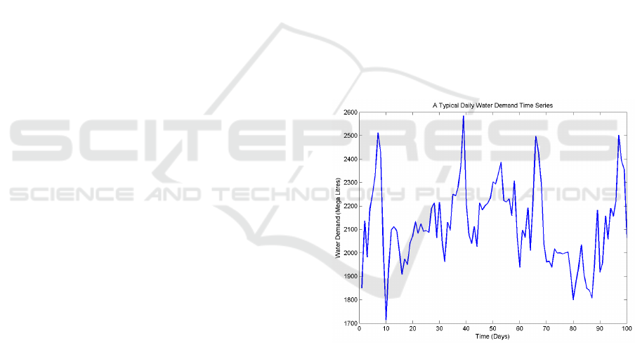
Figure 3 depicts a snapshot of this water demand time

series. The water demand time series used in this

study has a total of 3 470 instances of data with daily

frequency, but the snapshot in ﬁgure 3 shows only 100

data instances – with daily fequency – in the interest

of clearer visualization.

Figure 3: A snapshot of the water demand time series (with

daily frequency) used in this study. It is characterised by

non-linearity and arbitrary complexity.

A conventional neural network model would,

therefore, end up with a total of ﬁve inputs (four wa-

ter demand ﬁgures and one population ﬁgure) and one

output (water demand ﬁgure of the ﬁfth day). An au-

toencoder network, as mentioned before, is trained to

recall its inputs and, thereafter, expected to present

the same inputs in the output space. This implies that

the variable of interest (water demand ﬁgure of every

ﬁfth day), has to form part of the input space. The au-

toencoder network used in this study, therefore, ends

up with a total of six inputs and six outputs.

SIMULTECH 2016 - 6th International Conference on Simulation and Modeling Methodologies, Technologies and Applications

234

4.3 Data Treatment

The data used in this study is treated in two ways;

data division and data normalization. The data is di-

vided in accordance with the cross-validation tech-

nique, where there is a total of three data sets: the

training set, the validation set, and the testing set.

Table 1: The Division of Data into Three Separate Sets.

Data Set Distribution Total

Training 294 × 6 1 764

Validation 201 × 6 1 206

Testing 199 × 6 1 194

The training set is used to optimize the model,

with close monitoring achieved through the valida-

tion set. The testing set is used to evaluate the per-

formance of the trained network, and determine if it

has generalization ability. The resulting data distribu-

tion is summarized in table 1. This distribution of data

is exactly the same is the one reported in Msiza’s lat-

est work on water demand predictive modelling using

neural computing (Msiza et al., 2008).

Data normalization is done so as to ensure that all

the instances of data are of the same order of magni-

tude and hence simplify the network training process.

The largest value in the dataset is scaled to one, and

the smallest value is scaled to zero. This normaliza-

tion is achieved by making use of the following rela-

tionship:

norm

x − x

min

max

− x

min

(3)

where x

norm

is the normalized version of x, x

min

is the

smallest instance in the dataset, and x

max

is the largest

instance in the dataset.

4.4 Hidden Nodes Experiment

Now that both the input and the output space have

been determined, there is a need to determine the op-

timum number of nodes in the hidden unit, in order

to complete the architecture of the network. This is

done by making use of ∆E between the training set

and the validation set. Because this is an autoencoder

network with six nodes in both the input and output

units, the number of nodes in the hidden unit has to

be any ﬁgure between one and ﬁve. The training set

is used to – under supervision – optimize the network,

while the validation set is used to ensure that the av-

erage validation error,

validation

, is less than or equal

to the training error, E

training

The average training error is the error between the

target output and the output produced by the autoen-

coder network, when presented with training data.

Similarly, the average validation error is the error be-

tween the target output and the output estimated by

the autoencoder network, when presented with val-

idation data. A validation error that is less than or

equal to the training error implies that the network

does have the ability to generalize, that is, it can make

reliable estimates when presented with previously un-

seen data.

To the contrary, a validation error that is greater

than the training error means that the network has

poor generalization ability. The error is computed as

the absolute value of the Residual divided by the tar-

get value, expressed as a percentage. The Residual

is a statistical term used for the arithmetic difference

between a predicted value and its targeted value (Utts

and Heckard, 2015). The mathematical deﬁnition of

this error (E) is as follows:

E =

− y

× 100% (4)

where y

is the output predicted by the trained net-

work, and y

is the targeted output. The average of

this error is deﬁned as:

E =

∑

k=1



)

− (y

)



)

× 100% (5)

where (y

)

and (y

)

are – in the given order – the

target and the predicted output for the k

instance of

data, and M is the total number of instances in a given

data set.

Nabney’s Netlab Toolbox (Nabney, 2004) is used

to create the autoencoder network using the MLP ar-

chitecture. It is trained using the scaled conjugate gra-

dient (SCG) algorithm with a linear activation func-

tion, for 5 000 cycles. The average validation error

is computed for each value of N

hidden

. Recall that the

validation error is just the error deﬁned in equation 4,

for the validation set. The word “average” is used to

indicate the validation errors of all the data instances

have been added up, and divided by the total number

of instances in the dataset, expressed as a percentage,

as deﬁned in equation 5. The results obtained from

this experiment are summarized in table 2, where it

is apparent that the optimum number of nodes in the

hidden unit is ﬁve.

Figure 4 shows plots of both the actual and pre-

dicted outputs obtained from the autoencoder network

during the training process; while ﬁgure 5 shows plots

of both the actual and predicted outputs obtained from

the trained autoencoder network, when exposed to the

validation data set.

Autoencoder Networks for Water Demand Predictive Modelling

235

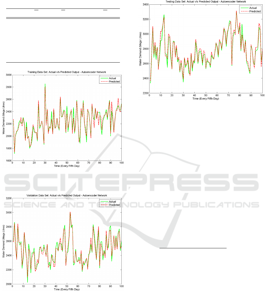
Table 2: The Results of the Hidden Nodes Experiment.

hidden

training

validation

∆E

1 4.9604% 4.9731% −0.0127%

2 4.6435% 3.9704% +0.6731%

3 2.5479% 2.1436% +0.4043%

4 1.7653% 1.4940% +0.2713%

5 1.3273% 1.2202% +0.1071%

Figure 4: Autoencoder network - predicted output (dotted

plot), from the training data set, on the same system of axes

with the target/actual output (solid plot).

Figure 5: Autoencoder network - predicted output (dotted),

from the validation data set, on the same system of axes

with the target/actual output (solid)

4.5 Performance Evaluation

Following the successful completion of the process of

determining the optimum number of nodes in the hid-

den unit, it then becomes necessary to evaulate the

performance of this optimized network under the ex-

posure of the testing data set. The average error in-

Figure 6: Autoencoder network - predicted output (dotted

plot), from the testing data set, on the same system of axes

with the target/actual output (solid plot).

troduced in equation 5, and the time taken by the op-

timized autoencoder network to produce an output –

given a single instance of input data – are readily us-

able as measures of perfomance. It is, however, nec-

essary to introduce an additional measure that should

indicate the accuracy of the optimized network.

The accuracy of an optimized network can – de-

pending on the application at hand – be evaluated in a

number of ways. This manuscript introduces a ﬁgure

of tolerance, T . If the predicted water demand value

is equal to the target value, plus or minus the ﬁgure

of tolerance, then it is counted as accurate. The total

of the counted accurate values is then divided by the

total number of data points (199) in the testing set and

multiply it by a hundred, to express it as a percentage.

This relationship is depicted in equation 6.

A =

∀



− y

)



≤ T : Count(y

)

Count(y

)

× 100% (6)

According to the South African Department of

Water and Environmental Affairs (previously known

as the Department of Water Affairs and Forestry), the

water services sector represents an overall demand

that is 19% of the total water supplied (Msiza et al.,

2007). This implies that 19% of the water supplied

is consumed by the water supplier itself. An analy-

sis of the overall data set used in this study indicates

that the average annual water demand is 2 700 Mega

Litres, and 19% of this ﬁgure works out to 513 Mega

Litres. Using equation 6 – with the worked out value

of T = 513 Mega Litres – the optimized autoencoder

network, an accuracy of 100% is obtained. Figure 6

depicts – on the same system of axes – the autoen-

coder network predicted time series, versus the actual

time series.

SIMULTECH 2016 - 6th International Conference on Simulation and Modeling Methodologies, Technologies and Applications

236

5 CONVENTIONAL NEURAL

NETWORK

IMPLEMENTATION

In order to benchmark the performance of this autoen-

coder network, a conventional neural network is im-

plemented and exposed to the same data sets.

5.1 Model Inputs and Outputs Selection

This conventional network – unlike the autoencoder

network – has a total of ﬁve inputs (water demand

values of the past four days and the population ﬁgure)

and one output (water demand value of the ﬁfth day).

As mentioned before, the autoencoder network has an

additional input variable because the required output

(water demand ﬁgure of the ﬁfth day) has to form part

of the input vector.

5.2 Hidden Nodes

With the autoencoder network, the optimum number

of hidden nodes was determined in an experimental

fashion, but with a conventional network that process

is done through the guidance of Kolmogorov’s the-

orem on multi-layer neural networks (Msiza et al.,

2011). This theorem suggests that, during the process

of training a conventional multi-layer neural network

model, the number of nodes in the hidden unit should

be twice the number of parameters in the input unit.

The conventional network, for that reason, ends up

with a total of ten nodes in the hidden unit (because

there is a total of ﬁve nodes in the input unit).

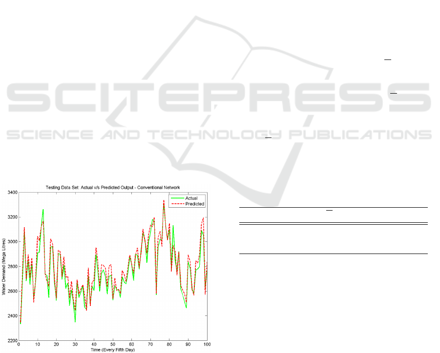
Figure 7: Conventional network - predicted output (dotted

plot), from the testing data set, on the same system of axes

with the target/actual output (solid plot).

5.3 Performance Evaluation

Like the autoencoder network, this conventional net-

work is trained through the use of the SCG algorithm

with a linear activation function, for 5 000 cycles.

This is after using the same data treatment techniques

used in the case of the autoencoder network. Figure 7

shows a time series predicted by the trained conven-

tional network, versus the actual time series, when

exposed to the testing data set. Using the same per-

formance indicators as in the case of the autoencoder

network, the next section carries out a comparison of

the two networks.

6 COMPARING THE

PERFORMANCE OF THE TWO

NETWORKS

Table 3 summarizes the comparison, in performance,

between the conventional and the autoencoder net-

work. These two networks are compared in terms of

accuracy (A), average prediction error (E), the time it

takes to generate a single output, and dimensionality

(D). Ideally, a better perfoming network should have

a higher value of A, and lower values of E, time, and

D. From table 3, it is easy to conclude that the autoen-

coder network is better than the conventional network.

This is due to the fact that the autoencoder has a lower

value of E and D, while they have the same value for

A. The conventional network only – slightly – outper-

foms the autoencoder network in terms of time.

Table 3: Comparison between the Conventional Network

(CN) and the Autoencoder Network (AN).

Model A E Time (s) D

CN 100% 1.99% 3.70 × 10

−5

AN 100% 1.25% 3.72 × 10

−5

7 CONCLUSIONS AND FUTURE

WORK

The purpose of the work presented in this manuscript

was to interrogate the usability of autoencoder neural

networks in predicting a water demand time series.

The choice of autoencoder networks was inspired by

the ideal of having a network that has low dimension-

ality, less complexity, high accuracy, and good gen-

eralization ability. This study was conducted using

Autoencoder Networks for Water Demand Predictive Modelling

237

real data obtained from Rand Water, a bulk water sup-

plier in South Africa. This data was split into three

sets: one to train the network, another to validate

the training process, and the last one to evaluate the

performance of the trained network. Using a simple

and computationally inexpensive approach to deter-

mine the optimum number of nodes in the hidden unit,

the autoencoder ended up with a dimensionality of 5.

This was exactly half of the dimensionality of the con-

ventional network – informed by Kolmogorov’s the-

orem – with which it was compared. Both networks

registered a prediction accuracy of 100%, however the

autoencoder network had a lower average prediction

error. The conventional network slightly outperfomed

the autoencoder network in terms of the time taken

to generate data in the output layer. However, the

fact that the autoencoder network has a dimension-

ality that is signiﬁcantly less than that of the conven-

tional network, makes it a better performing model.

Because both models registered 100% accuracy, it

would be useful to introduce variations on the data,

then evaluate the performance of the two models. Ex-

posing both models to various combinations of train-

ing algorithms and activation functions could, could

also be helpful. In addition, it could be useful to in-

troduce more neural network architectures, in order

to have a rich pool of model comparison. All these

suggestions could form part of possible future work.

ACKNOWLEDGEMENTS

The authors hereby acknowledge and thank Thomas

Phetlha, from Rand Water, for the water demand data.

REFERENCES

Bougadis, J., Adamowski, K., and Diduch, R. (2005).

Short-term Municipal Water Demand Forecasting. In

Hydrological Processes 19. pp 137-148.

Cooks, J. (2004). 100 Years of Excellence 1903-2003. Rand

Water, Johannesburg, 1st edition.

Hessel, M., Borgatelli, F., and Ortalli, F. (2014). A Novel

Approach to Model Design and Tuning through Auto-

matic Parameter Screening and Optimisation - Theory

and Application to a Helicopter Flight Simulator Case

Study. In 4th Intl. Conf. on Simulation & Modelling

Methodologies, Technol., and Appl. pp 24–35.

Jain, A., Varshney, A. K., and Joshi, U. C. (2001). Short-

term Water Demand Forecast Modelling at IIT Kanpur

Using Artiﬁcial Neural Networks. In IEEE Trans. on

Water Resources Management 15. pp 299-321.

Leke-Betechuoh, B., Marwala, T., and Tettey, T. (2006).

Autoencoder Networks for HIV Classiﬁcation. In

Current Science 91. pp 1467-1473.

Marivate, V. N., Nelwamondo, F. V., and Marwala, T.

(2008). Investigation into the Use of Autoencoder

Neural Networks, Principal Component Analysis and

Support Vector Regression in Estimating Missing HIV

Data. In 17th World Congress of the Intl. Federation

of Automatic Control. pp 682-689.

Marwala, T. (2016). Handbook of Machine Learning:

Foundation of Artiﬁcial Intelligence. Imperial College

Press, London, (Accepted for Publication) edition.

Msiza, I. S., Nelwamondo, F. V., and Marwala, T. (2007).

Water Demand Forecasting Using Multi-layer Percep-

tron and Radial Basis Functions. In IEEE Intl. Joint

Conf. on Neural Networks. pp 13-18.

Msiza, I. S., Nelwamondo, F. V., and Marwala, T. (2008).

Water Demand Prediction Using Artiﬁcial Neural

Networks and Support Vector Regression. In Journal

of Computers 3. pp 1–8.

Msiza, I. S., Szewczyk, M., Halinka, A., Pretorius, J. H.,

Sowa, P., and Marwala, T. (2011). Neural Net-

works on Transformer Fault Detection: Evaluating

the Relevance of the Input Space Parameters. In

IEEE PES Power Systems Conf. & Exposition. DOI:

10.1109/PSCE.2011.5772567.

Nabney, I. T. (2004). Algorithms for Pattern Recognition.

Springer, Heidelberg, 4th edition.

Nelwamondo, F. V., Golding, D., and Marwala, T. (2013).

A Dynamic Programming Approach to Missing Data

Estimation Using Neural Networks. In Information

Sciences 237. pp 49-58.

Solanki, A., Agrawal, H., and Khare, K. (2015). Predic-

tive Analysis of Water Quality Parameters using Deep

Learning. In Intl. Journal of Computer Appl. 125. pp

29-34.

Thompson, B. B., Marks, R. J., Choi, J. J., El-Sharkawi,

M. A., Huang, M.-Y., and Bunje, C. (2002). Implicit

Learning in Autoencoder Novelty Assessment. In

IEEE Intl. Joint Conf. on Neural Networks. pp 2878–

2883.

Utts, J. M. and Heckard, R. F. (2015). Mind on Statistics.

Cengage Learning, Stanford, 5th edition.

van Deventer, V. and Mojapelo-Batka, M. (2013). A Stu-

dent’s A-Z of Psychology. Juta & Company, South

Africa, 2nd edition.

Yuan, Y. and Jia, K. (2015). A Water Quality Assessment

Method Based on Sparse Autoencoder. In IEEE Intl.

Conf. on Signal Processing, Communications & Com-

puting. pp 1-4.

Zhiyin, W., Long, Y., and Shengwei, T. (2015). Water Body

Extraction Method Based on Stacked Autoencoder. In

Journal of Computer Appl. 35. pp 2706-2709.

SIMULTECH 2016 - 6th International Conference on Simulation and Modeling Methodologies, Technologies and Applications

238