
Symplectic Discretization Methods for Parameter Estimation of a
Nonlinear Mechanical System using an Extended Kalman Filter
Daniel Beckmann, Matthias Dagen and Tobias Ortmaier
Institute of Mechatronic Systems, Leibniz Universit¨at Hannover, Appelstraße 11a, Hanover, Germany
Keywords:
Online Estimation, Kalman Filter, Discretization Methods, Mechanical System.
Abstract:
This paper presents two symplectic discretization methods in the context of online parameter estimation for a
nonlinear mechanical system. These symplectic approaches are compared to established discretization meth-
ods (e.g. Euler Forward and Runge Kutta) regarding accuracy and computational effort. In addition, the
influence of the discretization method on the performance of an augmented Extended Kalman Filter (EKF) for
parameter estimation is analyzed. The methods are compared with a nonlinear mechanical simulation model,
based on a belt-drive system. The simulation shows improved accuracy using simplectic integrators in com-
parison to the conventional methods, with almost the same or lower computational cost. Parameter estimation
based on the EKF in combination with the simplectic integration scheme leads to more accurate values.
1 INTRODUCTION
Online state and parameter estimation is important in
various fields, e.g. adaptive control, predictive main-
tenance and other engineering areas. Especially for
stochastic state space systems the state-augmented
Extended Kalman Filter (EKF) is a widely used ob-
server to estimate states and parameters in real time
(Grewal and Andrews, 2008). In particular it is used
in several industrial applications for control, diagnos-
tics, sensor data fusion and signal processing (Auger
et al., 2013; Szabat and Orlowska-Kowalska, 2012).
The EKF uses linearized system and measurement
models at the current estimate using partial deriva-
tions (Welch and Bishop, 2006). This can lead to
poor performance when models are highly nonlinear,
because the covariance is propagated through the lin-
earization. Furthermore, using the EKF as parame-
ter estimator for linear systems can lead to biased pa-
rameter estimates, if covariance values are incorrect
(Ljung, 1979).
Moreover, accurate state and parameter estimation
by the observer also requires precise system modeling
and proper initial values. Traditionally, mechanical
systems are modeled using continuous-time methods
(e.g. Lagrange’s equations) to obtain the equations
of motion. The resulting equations (typically second
order ordinary differential equations) are transformed
into continuous-time state space form. A continuous-
discrete Extended Kalman Filter can be used to solve
the continuous-time state space system and its covari-
ance propagation numerically (Sch¨utte et al., 1997;
Bohn, 2000).
Another approach uses explicit discretization
methods to find an analytical expression of a discrete-
time model (Riva et al., 2015). The most common
practice to find the analytical expression is to use the
Euler Forward method with the discretization order
one. The Jacobian of the discrete-time model, which
can be calculated analytically and evaluated at the cur-
rent estimate, is used to propagate the error covari-
ance matrix.
However, using explicit discretization methods
can lead to unstable discrete-time models, if the sam-
pling time is too large compared to the time constant
of the continuous model. In many applications, the
sampling time is fixed by the used hardware (e.g. for
industrial application usually 1 ms). Therefore, the
way to obtain a stable discrete-time model is to raise
the order of the discretization method. Increasing
the order results in higher accuracy of the discrete-
time solution, but the computational effort will be in-
creased, too. In general, a trade-off between calcu-
lation time and accuracy needs to be found. In fact,
there are many other implicit methods to calculate
a discrete-time solution (like collocation or implicit
Runge-Kutta methods), but usually all of these meth-
ods need an iterative gradient-based optimization al-
gorithm (e.g. Newton-Raphson method) at each time
step. Due to this fact, this paper focuses explicit (and
Beckmann, D., Dagen, M. and Ortmaier, T.
Symplectic Discretization Methods for Parameter Estimation of a Nonlinear Mechanical System using an Extended Kalman Filter.
DOI: 10.5220/0005973503270334
In Proceedings of the 13th International Conference on Informatics in Control, Automation and Robotics (ICINCO 2016) - Volume 1, pages 327-334
ISBN: 978-989-758-198-4
Copyright
c
2016 by SCITEPRESS – Science and Technology Publications, Lda. All rights reserved
327

semi implicit) methods.
As already mentioned, the most common dis-
cretization method is the Euler Forward approach.
Higher order methods are Heun method (order two),
Simpson rule (order three) and classical Runge Kutta
method (order four). In the context of online param-
eter estimation for a mechanical system, this paper
presents the first application and results using semi
implicit Euler and leapfrog discretization method.
Both approaches belong to the scheme of symplectic
integrators (Hairer et al., 2006). This paper compares
these methods to the conventional methods mentioned
above, in context of accuracy and computing time of
the discrete-time model (and its Jacobian). In addi-
tion, the influence of the discretization method to the
accuracy of estimated parameter using an EKF is ana-
lyzed. The model, which is used for the investigation,
is based on a nonlinear belt-drive system for position-
ing tasks. The model parameters are identified using
Grey-box identification methods.
The paper is organized as follows. Section 2.1
shortly presents the algorithm of EKF and state-
augmented EKF. The discretization methods are in-
troduced in section 2.2. In section 3 the testbed and its
modeling are given. The simulation results are shown
in section 4. The paper closes with a conclusion in
section 5.
2 METHODS
2.1 Extended Kalman Filter
Consider the following nonlinear discrete-time state
space model with additive noise:
x
k
= f (x
k−1
,θ
k−1
,u
k
) + w
k−1
, (1)
y
k
= h(x
k
,θ
k−1
) + v
k
, (2)
with the state vector x
k
∈ R
n
x
, the unknown parame-
ter vector θ
k
∈ R
n
θ
, the input u
k
∈ R
n
u
and the output
y
k
∈ R
n
y
. The (non)linear system and measurement
functions are described by f and h. Process and mea-
surement noises are represented by w
k−1
∼ N (0,Q
x
)
and v
k
∼ N (0,R
k
), with Q
x
and R
k
the process and
measurement noise covariance matrices, respectively.
The initialization of EKF is defined by setting the
start values for the state vector x
0
and its error covari-
ance matrix P
0
:
ˆx
0
= x
init
∈ R
n
x
and
P
0
= P
init
∈ R
n
x
×n
x
.
(3)
In addition Q
x
∈ R
n
x
×n
x
and R
k
∈ R
n
y
×n
y
need to be
set. These matrices are assumed to be diagonal. The
recursion of the EKF starts with the time update step
as follows:
ˆx
−
k
= f ( ˆx
k−1
,θ
k−1
,u
k
) , (4)
P
−
k
= A
k
P
k−1
A
T
k
+ Q
x
, (5)
with
A
k
=
∂f
∂x
k
x
k
= ˆx
−
k
,θ
k−1
,u
k
∈ R
n
x
×n
x
. (6)
After this prediction step, the correction step can be
calculated as:
K
k
= P
−
k
H
T
k
H
k
P
−
k
H
T
k
+ R
k
, (7)
ˆx
k
= ˆx
−
k
+ K
k
y
k
− h(ˆx
−
k
,θ
k−1
)
, (8)
P
k
= (I − K
k
H
k
)P
−
k
, (9)
with
H
k
=
∂h
∂x
k
x
k
= ˆx
−
k
,θ
k−1
∈ R
n
y
×n
x
. (10)
In order to estimate unknown parameters, the state
vector can be augmented to
(a)
x
k
= [x
T
k
, θ
T
k
]
T
∈
R
n
a
=n
x
+n
θ
which leads to a new nonlinear discrete-
time state space model as:
x
k
θ
k
|
{z}
(a)
x
k
=
f (x
k−1
,θ
k−1
,u
k
)
θ
k−1
|
{z }
˜
f(
(a)
x
k−1
,u
k
)
+
w
k−1
ω
k−1
, (11)
y
k
=
˜
h
(a)
x
k
+ v
k
, (12)
with the modified system and measurement functions
˜
f and
˜
h. The dimension is increased by the number
of unknown parameters. Then the initialization of the
EKF is now defined as:
(a)
ˆx
0
=
x
T
init
, θ
T
init
T
∈ R
n
a
and
(a)
P
0
=
P
init
0
0 Θ
init
∈ R
n
a
×n
a
.
(13)
Furthermore, the dimension of process noise covari-
ance matrix is also increased to:
(a)
Q =
Q
x
0
0 Q
θ
∈ R
n
a
×n
a
, (14)
where Q
θ
∈ R
n
θ
×n
θ
describes the covariance matrix of
pseudo noise ω
k−1
for the parameter estimation and is
also assumed to be diagonal.
2.2 Discretization Methods
Consider the following nonlinear continuous-time
state equation
˙x = f (x, u) , (15)
ICINCO 2016 - 13th International Conference on Informatics in Control, Automation and Robotics
328

with the state vector x and the control vector u. Us-
ing the Euler Forward method is the simplest way to
obtain a discrete-time state equation which is given
by
x
k
= x
k−1
+ T
S
f (x
k−1
,u
k−1
) , (16)
where T
S
is defined by the sampling time. The order
of the Euler Forward method is one. However, due to
the order one, the method is often not accurate enough
to reproduce the true dynamics of the continuous-time
model. In addition, the numerical solution can be un-
stable, especially for stiff equations. To obtain a sta-
ble numerical solution, either the sampling time can
be reduced or the order of the discretization method
has to be raised. In many industrial applications the
sampling time is limited by the hardware. Raising the
order leads to Runge Kutta methods. For example, the
Heun method has the order two and is given by:
˜x
k
= x
k−1
+ T
s
f (x
k−1
,u
k−1
) ,
x
k
= x
k−1
+
T
s
2
f (x
k−1
,u
k−1
)
+ f ( ˜x
k
,u
k
)
.
(17)
It is based on the prediction of the state vector ˜x
k
in
the first step and a correction in the second step. A
method of order three, is given based on the Simpson
rule (or Runge Kutta three). The calculation is defined
by:
a
1
= f(x
k−1
, u
k−1
),
a
2
= f
x
k−1
+
T
S
2
a
1
,u
k−1/2
,
a
3
= f (x
k−1
− T
S
a
1
+ 2T
S
a
2
,u
k
) ,
x
k
= x
k−1
+
T
S
6
(a
1
+ 4a
2
+ a
3
) ,
(18)
where u
k−1/2
is given by the mean value between u
k−1
and u
k
. The classical Runge Kutta method with its
order four is given by:
a
1
= f(x
k−1
, u
k−1
),
a
2
= f
x
k−1
+
T
S
2
a
1
,u
k−1/2
,
a
3
= f
x
k−1
+
T
S
2
a
2
,u
k−1/2
,
a
4
= f (x
k−1
+ T
S
a
3
,u
k
) ,
x
k
= x
k−1
+
T
S
6
(a
1
+ 2a
2
+ 2a
3
+ a
4
) .
(19)
All these methods are explicit, i.e. only previous val-
ues of the state vector x are used to calculate the actual
value. The input variable u is used at time step k and
k− 1, which is usually available in many applications.
However,each of the described methods can result
in an unstable solution. Raising the order is an option
to obtain a stable equation, but it also increases the
computational time. Hence, a trade-off between ac-
curacy and computing time has to be found. In fact,
there are many other methods for discretization. Es-
pecially for mechanical systems, symplectic integra-
tion methods are notable and are discussed in the fol-
lowing.
The semi implicit Euler method (also called sym-
plectic Euler) is the simplest way to obtain a symplec-
tic integration (Niiranen, 1999). It is a modification of
the Euler Forward method to solve Hamilton’s equa-
tion and the results are more accurate than classical
approaches. However, this method requires a pair of
differential equations of the form
ds
dt
= ˙s = Φ(v) ,
dv
dt
= ˙v = Ψ(s,v) ,
(20)
where s represents a position vector and v the corre-
sponding velocity vector. These equations are typical
for classical mechanics. Using the symplectic Euler
method leads to the discrete-time equations
v
k
= v
k−1
+ T
s
Ψ(s
k−1
,v
k−1
) ,
s
k
= s
k−1
+ T
s
Φ(v
k
) .
(21)
It is important to note, that the velocity vector is cal-
culated first, using only old values of velocity and po-
sition. In the second step, the position is calculated
using the new value of velocity and the old position
value. The simplectic Euler method has order one. A
second order method, called leapfrog integration, is
given by two steps of symplectic Euler:
v
k−1/2
= v
k−1
+
T
s
2
Ψ(s
k−1
,v
k−1
) ,
s
k−1/2
= s
k−1
+
T
s
2
Φ
v
k−1/2
,
s
k
= s
k−1/2
+
T
s
2
Φ
v
k−1/2
,
v
k
= v
k−1/2
+
T
s
2
Ψ
s
k
,v
k−1/2
.
(22)
The mentioned discretization methods in combination
with the parameter estimation are evaluated based on
a mechanical testbed model, which is described in the
following section.
3 TESTBED AND MODELING
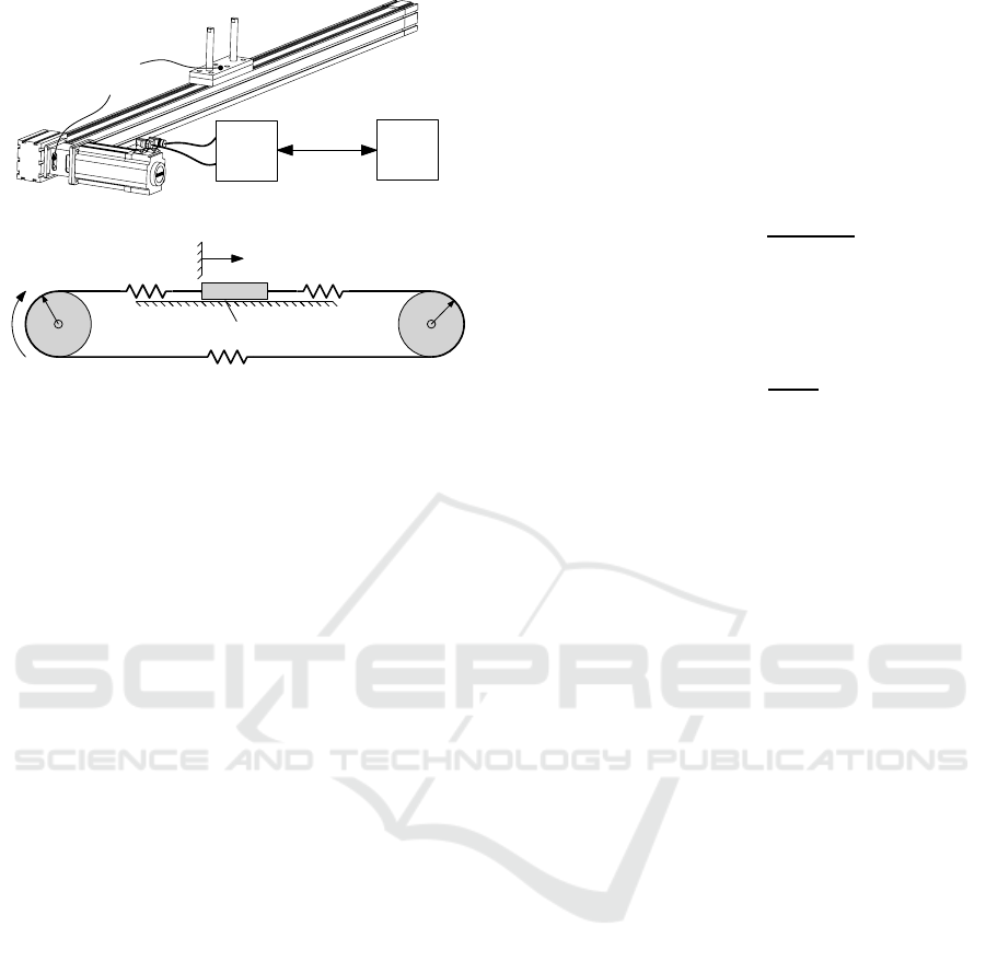
The structure of the testbed is shown in Figure 1(a)
and consists of a belt-drive for positioning tasks with
Symplectic Discretization Methods for Parameter Estimation of a Nonlinear Mechanical System using an Extended Kalman Filter
329
servo
inverter
variable mass m
pulley radius r
servo
motor
PLC
ETHERCAT
R
bus @ 1 kHz
(a) Structure of the testbed with commercial hardware.
I
1
I
2
≈ 0
ϕ, ˙ϕ, ¨ϕ
r
1
r
2
τ
m
µ
v
, µ
c
z, ˙z, ¨z
m
c
1
(z) c
2
(z)
c
3
(b) Schematic of mechanical model.
Figure 1: Structure and mechanical model of the testbed.
variable transporting masses. It is directly driven by a
permanent magnet synchronous motor and a servo in-
verter. The latter is connected via a real-time ETHER-
CAT
R
bus to a programmable logic controller (PLC).
The motor is controlled by a conventional cascade
structure with P- and PI-feedback controller for motor
position and speed (filtered position derivative).
The main focus in industrial motion design is time
optimality, so acceleration trapezoid profiles (ATP)
are used to calculate the setpoint values for the motion
control. Due to the exploitation of at least one limita-
tion of velocity, acceleration and jerk (v
max
, a
max
and
j
max
) at each instant of a movement, these profiles
guarantee the shortest possible traveling time (Bia-
giotti and Melchiorri, 2008). In this context, the jerk
time is defined as t
j
= a
max
j
−1
max
.
A mechanical model is given by a flexible body
system with two degrees of freedomand the following
equations of motion (see Figure 1(b))
F = M ¨q+ D ˙q+ C (q)q+ H (˙q), (23)
with the generalized coordinate vector q = [ϕ, z]
T
and
M =
I
m
+ I
1
0
0 m
, D =
dr
2
1
−dr
1
−dr
1
d + µ
v
,
(24)
C (q) =
c
eff
(z)r
2
1
−c
eff
(z)r
1
−c
eff
(z)r
1
c
eff
(z)
, (25)
H (˙q) =
0
µ
c
tanh(k˙z)
, F =
τ
m
0
. (26)
Here, τ
m
is the actual motor torque, r
1
is the pulley
radius, ϕ and z the motor angle and load position, re-
spectively. The parameters in the mass matrix M are
the motor inertia I
m
, the inertia of the connection be-
tween motor and belt drive I
1
and the load mass m.
The elements of the damping matrix D are the belt
damping d (not shown in the figure) and a viscous
friction coefficient on the sliding mass µ
v
. The stiff-
ness matrix C contains the position depending belt
stiffness c
eff
(z).
The belt stiffness is calculated by the series and
parallel connection of the spring constants of each
belt segment (see Figure 1(b)):
c(z) = c
1
(z) +
c
2
(z)c
3
c
2
(z) + c
3
, (27)
where c
1
(z) and c
2
(z) are functions of the load po-
sition (Nevaranta et al., 2015). An approximation of
(27) is given by:
c
eff
(z) = c
spec
1+
1
z
0
+ z
≈ c(z), (28)
where c
spec
is a belt specific spring constant and z
0
a position constant depending on the initial value
of load position z. In addition to the viscous fric-
tion at the sliding mass, an approximation of a static
Coulomb friction model (parameter µ
c
and k) is as-
sumed in the nonlinear term H (˙q).
Using the state space vector x = [q
T
, ˙q
T
]
T
=
[ϕ, z,
˙
ϕ, ˙z]
T
, the system can be transformed into the
continuous-time state space equation
˙x =
x
3
x
4
(I
m
+ I
1
)
−1
(τ
m
− r
1
F
d
− r
1
F
c
)
m
−1
(F
d
+ F
c
− F
f
)
, (29)
with
F
d
= d(x
3
r
1
− x
4
),
F
c
= c
eff
(x
2
)(x
1
r
1
− x
2
),
F
f
= µ
v
x
4
+ µ
c
tanh(kx
4
).
(30)
The motor angle and its velocity can be measured,
which leads to the following measurement function:
y =
1 0 0 0
0 0 1 0
x. (31)
Due to the transformation to state space, the pair of
equations needed for the symplectic integration meth-
ods is already given.
The parameter values of the continuous-time state
space model are identified using Grey-box identifica-
tion method (Bohlin, 2006) with a dynamic ATP (jerk
time < 10ms) to excite all system parameters. The re-
sult of the identification is shown in Figure 2, where
the measured signals and the model are compared.
The model fits the measured position with
99.88% and the measured velocity with 98.32%. The
identified parameter values are summarized in Ta-
ble 1.
ICINCO 2016 - 13th International Conference on Informatics in Control, Automation and Robotics
330
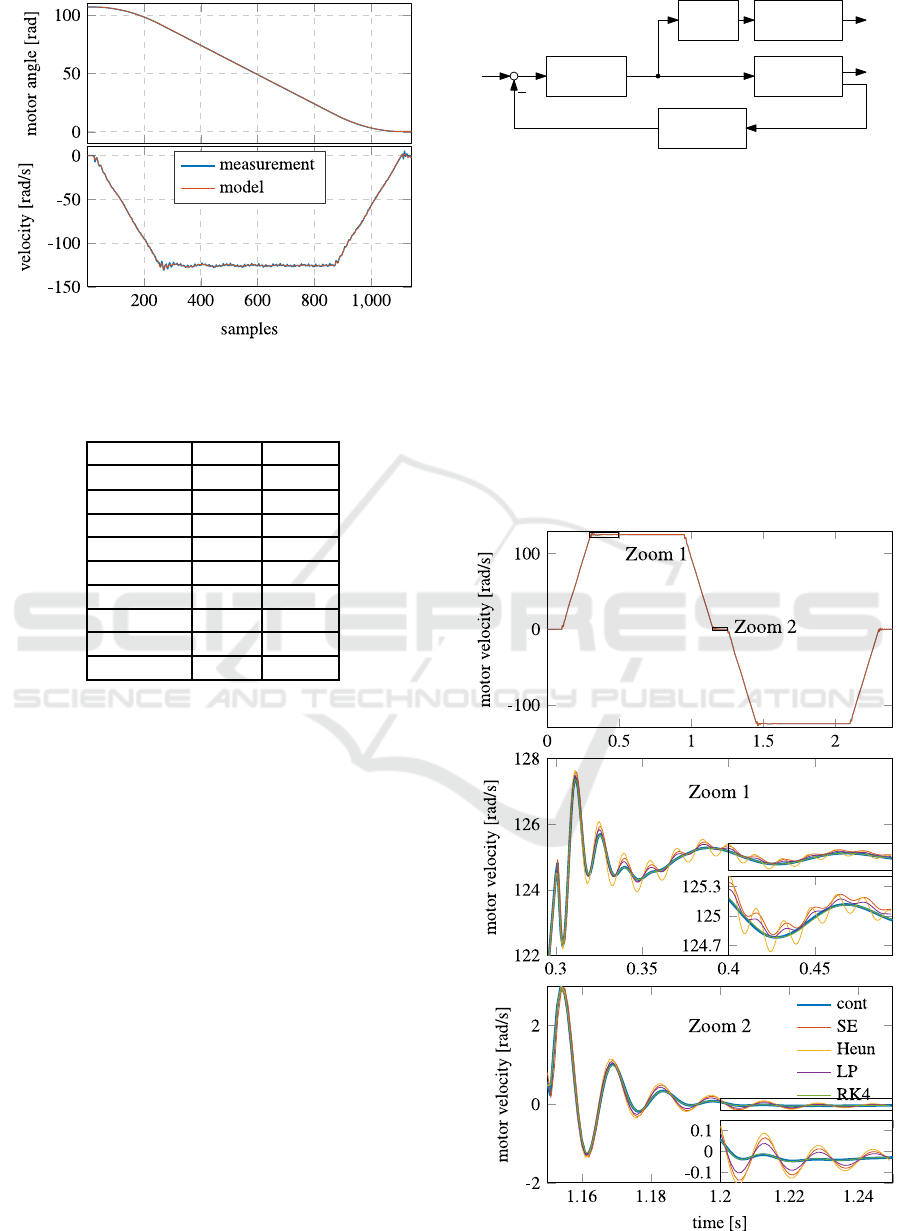
Figure 2: Comparison of measured motor angle and veloc-
ity against the identified model output.
Table 1: Identified parameter values.
Parameter Value Unit
I
m
+ I
1
13.00 kgcm
2
m 12.50 kg
c
spec
8.94 kN
d 97.66 Ns/m
µ
v
13.67 Ns/m
µ
c
28.13 N
k 50.00 s/m
z
0
0.13 m
r
1
15.90 mm
4 RESULTS
The simulation results are divided in two parts. The
first part focuses the comparison of the continuous-
time model and the described discretization methods,
which is pointed out in section 4.1. In the second
part, the influence of discretization method to param-
eter estimation based on an augmented EKF is shown
(section 4.2).
4.1 Comparison of Continuous and
Discrete Model
First, the simulation results using the mentioned
discretization methods (see section 2.2) are com-
pared to the continuous-time model. The sys-
tem structure and the data flow are shown in Fig-
ure 3. The time continuous solution is calculated us-
ing Dormand-Prince method with order eight (
ode8
-
solver in SIMULINK
R
) with a sampling frequency of
16 kHz. The discrete-time model is calculated with a
fixed sampling time of 1 ms. The exact analytical ex-
P/PI
Controller
Continuous
Model
Discrete
Model
Sample
& Hold
x
k
τ
m
Derivative
& Filtering
ϕ
x
Figure 3: Control structure.
pressions for the discrete-time models are generated
and optimized with the symbolic calculation software
MAPLE
R
.
The comparison of the discrete-time models is
shown in Figure 4. The first plot illustrates the con-
tinuous motor velocity for a given trajectory. To com-
pare the discretization methods, the system dynamics
need to be excited by the trajectory. The system vibra-
tions occur in areas where the acceleration changes
with small jerk time, exemplary shown in the detail
plots 1 and 2. The first detail plot (middle) shows the
behavior of the models near maximum velocity and
the second detail plot (bottom) at minimum velocity.
Figure 4: Comparison of discrete-time models.
Symplectic Discretization Methods for Parameter Estimation of a Nonlinear Mechanical System using an Extended Kalman Filter
331
Table 2: Comparison of computing cost and normalized
root mean square errors of discretization methods.
Mult Add Div NRMSE1 NRMSE2
EF 11 13 1 - -
SE 11 13 1 0.18 0.16
Heun 28 33 2 0.29 0.19
LP 22 31 2 0.13 0.14
RK3 53 58 3 0.07 0.08
RK4 64 72 4 0.06 0.07
The classical Runge Kutta method (RK4, green line)
fits the continuous signal (thick blue line) nearly per-
fect. In comparison to the Simpson rule, nearly no dif-
ference is visible, so this method is not shown in the
figure. Also not shown is the Euler Forward method
(EF), which is immediately unstable in this case. The
Heun method (yellow line) is able to capture the first
oscillations, but can’t reproduce the correct damping.
The symplectic integration methods are more ac-
curate than the Heun method reproducing the vibra-
tions. In fact, the RK4 method is still better than the
semi implicit Euler (SE, orange) and the leapfrog (LP,
purple), but the oscillations settle earlier in compari-
son to the Heun method. It should be noted, that the
SE method has the order one and the classical Heun
method has the order two. The normalized root mean
square errors (NRMSE) of the detail plots 1 and 2 are
printed in Table 2.
Furthermore, the number of operations for the nu-
merical evaluation of the discretization methods is an-
alyzed using the
cost
-function of MAPLE. The re-
sults are summarized in Table 2 and the abbrevia-
tions are defined as: additions (Add), multiplications
(Mult), and divisions (Div). As expected, the meth-
ods with order one have the same smallest number of
all numerical evaluations. Methods with second or-
der (Heun and LP) need one more division plus extra
multiplications and additions compared to order one
approaches. To reach Runge Kutta three method, the
effort is nearly doubled from methods with order two.
It is important to note, that the symplectic integra-
tors have another characteristic in this scenario. As
seen in Figure 4 (middle plot), the error between the
time continuous and the time discrete signal at con-
stant velocity is slightly higher compared to the es-
tablished methods. For example, the relative error
of symplectic Euler method at 0.8 s is about 0.05 %,
while the error of RK4 is lower than 0.002 %. How-
ever, due to the lower implementation effort, this error
is acceptable. In context of parameter estimation this
error has nearly no negative effect on the estimated
values, which is shown in the next section.
4.2 Parameter Estimation
Next, the discrete-time models are compared in order
to estimate parameters with an augmented EKF. The
parameters to estimate are chosen to be the specific
spring constant c
spec
and the belt damping d, because
these parameters mainly determine the oscillation be-
havior. For example, the estimated parameters can
be used for feedforward control methods to reduce or
eliminate these vibrations (e.g. flatness-based control
(Beckmann et al., 2015) or input-shaping technique
(
¨
Oltjen et al., 2015)).
The state space vector is augmented to
(a)
x
k
=
[ϕ, z,
˙
ϕ, ˙z, c
spec
, d]
T
. The discrete-time model from
the control structure (see Figure 3) is changed to an
augmented EKF. The continuous-time model is sim-
ulated without process noise, only the measurement
noise is added on the position and velocity. The EKF
parameters are set to:
Q
x
= P
init
= I10
−10
,
Q
θ
= diag(8× 10
−12
,8× 10
−12
),
Θ
init
= diag(1× 10
−1
,1× 10
−6
),
R = diag(1× 10
−9
,1× 10
−2
),
x
init
= [0,0,0, 0]
T
,
θ
init
=
0.2c
spec,ident
,2d
ident
T
=
1.79× 10
3
,195.32
T
.
(32)
The resulting parameter estimation with the aug-
mented EKF is shown in Figure 5. The first plot il-
lustrates the behavior of the estimated specific spring
constant and the second plot shows the belt damping.
The real simulated value is represented by the dashed
black line. With the Euler Forward method, the esti-
mates of both parameter are biased. However, due to
the feedback, the Kalman Filter can stabilize the un-
stable discrete-time solution. But, especially the belt
damping parameter is highly biased for this scenario
(about 8 times higher).
The best result for estimating the spring constant
is achieved by the RK4 method (RK3 method is sim-
ilar, therefore not shown in the picture). The rela-
tive error of the mean values of the last two seconds
is about 0.58% and 0.67 % for the RK4 and RK3
method. As seen from the results of the symplectic
integrators, it is obvious that the estimates are more
accurate than the Heun method. Even the SE method
(which has order one) reaches a slightly better esti-
mate in comparison to the Heun method (relative error
SE: 3.26 %, Heun: 3.61 %). The relative error of the
leapfrog method is about 2.48%. All relative errors
of the specific spring constant are printed in Table 3
marked as E1 (fifth column).
ICINCO 2016 - 13th International Conference on Informatics in Control, Automation and Robotics
332
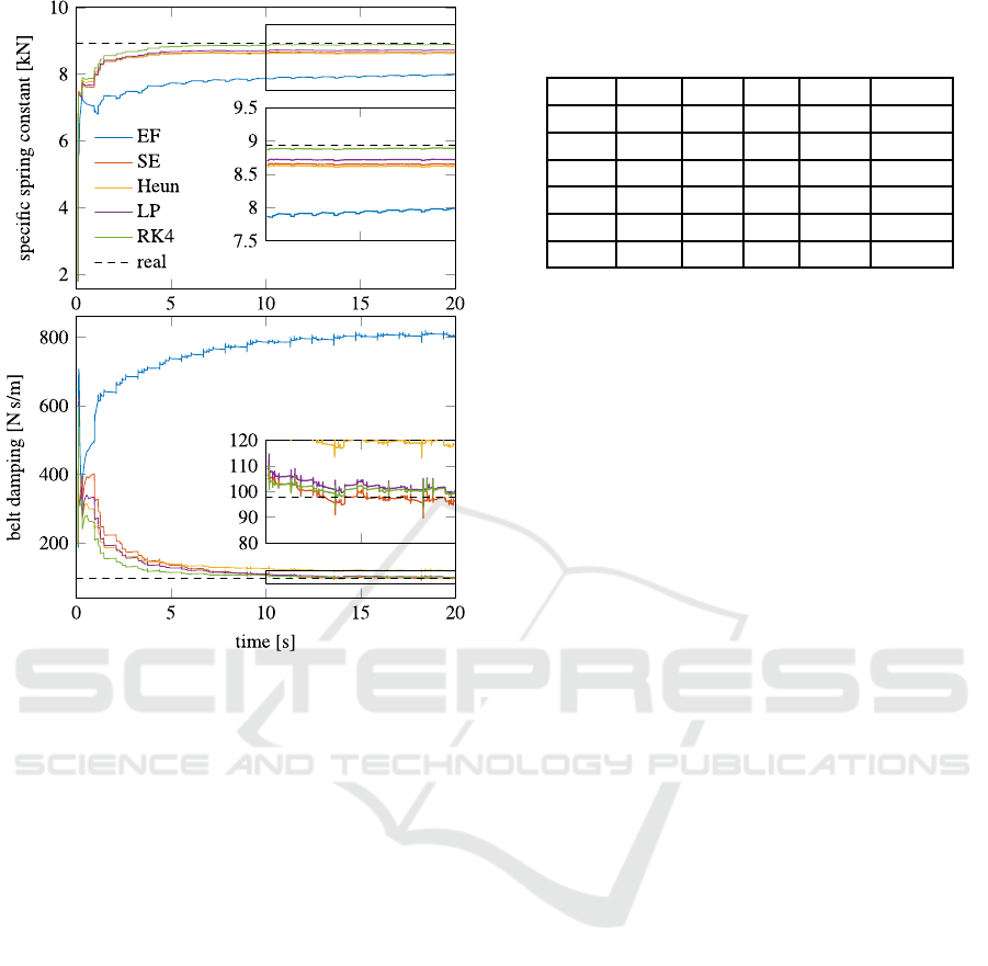
Figure 5: Parameter estimation of augmented EKF.
The belt damping constant is estimated well with
the SE, RK4, RK3 and LP method (relative error
lower than 5 %, see second picture and sixth column
of Table 3). Only the estimated value resulting from
the Heun method is higher than 20% compared to
the real value. It should be noted, that is EKF is
sub-optimal estimating parameters in the augmented
form, so the remaining parameter errors still depend
on the choice of covariance matrices. However, this
paper only compares the influence of the discretiza-
tion method to the parameter estimation.
To sum up, estimating the spring constant is possi-
ble with all tested discretization methods and the aug-
mented EKF. Even the unstable discrete-time model
using EF approach is able to estimate the spring con-
stant with a relative error of about 10 %. Estimating
the damping constant is more difficult and the param-
eter bias of the Euler Forward method is about 8 times
higher than the real value. Increasing the discretiza-
tion order by one (Heun method) leads to better re-
sults, but the estimated value is still about 20 % higher
than the real value. Only the RK4 (RK3) and the sym-
plectic methods are able to estimate the real damping
constant with a relative error lower than 5%.
However, comparing SE, LP, RK3 and RK4 re-
garding the computational costs for the augmented
Table 3: Comparison of computing cost and relative pa-
rameter estimation error of discretization method with aug-
mented state vector and calculating the Jacobian.
Mult Add Div E1 E2
EF 29 25 2 10.84 725.32
SE 44 29 2 3.26 1.18
Heun 147 110 4 3.61 21.90
LP 172 122 4 2.48 3.08
RK3 327 251 6 0.67 4.56
RK4 434 329 8 0.58 2.51
EKF (including the dicretization method and calcu-
lating its Jacobian), it is obvious, that the evaluation
counts, especially for RK3 and RK4, are highly in-
creased (see Table 3). The first reason is the increase
of the state vector and the calculation of the Jaco-
bian. The second reason is the more complex calcu-
lation of the Jacobian for the symplectic integrators,
that’s why the computational cost of first order meth-
ods differs (compare EF and SE). But, the parameter
estimation with the SE approach is much more accu-
rate compared to the EF method, especially for the
belt damping. Furthermore, the SE approach reaches
even better estimates than the Heun method, which
has second discretization order and needs more than
300% of multiplications. The multiplications needed
for the RK3 method are about 740% higher than the
SE method, but both methods estimate the parame-
ter with a relative error lower than 5 %, therefore in
the authors opinion the semi implicit Euler approach
is the best trade-off between accuracy and computa-
tional cost.
5 CONCLUSION
In this paper two symplectic discretization methods
are compared to established schemes in the context of
online parameter estimation. For the considered me-
chanical system these symplectic integrators are able
to solve the time continuous equations very accurately
and with the same (semi implicit Euler) or lower com-
puting cost (leapfrog method). In addition, the classi-
cal and commonly used Euler Forward method leads
to an unstable discrete-time system, while the SE
method with the same numerical evaluations results in
a stable discrete-time solution. However, if the high-
est accuracy is needed, Runge Kutta methods still pro-
vide the best results with the drawback of the highest
computational cost. Nevertheless, if the mechanical
system is poorly damped, the sampling time is fixed
and computing cost should be minimal (e.g. for real
time implementation), the simplectic integrators are
Symplectic Discretization Methods for Parameter Estimation of a Nonlinear Mechanical System using an Extended Kalman Filter
333

a possibility to provide adequate discrete-time mod-
els. In addition, the simplectic integration methods
are scalable, so mechanical systems with more than
two degrees of freedom can be calculated.
In the context of online parameter estimation us-
ing an augmented EKF, the advantage of symplectic
integration methods increases. The SE method out-
performed the Euler Forward method, where the es-
timated parameters are totally biased, while the re-
sults of the SE approach are more accurate (relative
error lower than 5 %). Furthermore, the estimation
results performed by the SE approach reach similar
(and higher) accuracy compared to the conventional
Runge Kutta methods needing a fraction of computa-
tional effort.
REFERENCES
Auger, F., Hilairet, M., Guerrero, J. M., Monmasson, E.,
and Orlowska-Kowalska, T. (2013). Industrial appli-
cations of the Kalman filter: A review. IEEE Transac-
tions on Industrial Electronics, 60:5458 – 5471.
Beckmann, D., Schappler, M., Dagen, M., and Ortmaier,
T. (2015). New approach using flatness-based con-
trol in high speed positioning: Experimental results.
In IEEE International Conference on Industrial Tech-
nology (ICIT), Sevilla.
Biagiotti, L. and Melchiorri, C. (2008). Trajectory Planning
for Automatic Machines and Robotics. Springer.
Bohlin, T. (2006). Practical Grey-box Process Identifica-
tion. Springer.
Bohn, C. (2000). Recursive Parameter Estimation for Non-
linear Continuous-Time Systems through Sensitivity-
Model-Based Adaptive Filters. PhD thesis, Depart-
ment of Electrical Engineering and Information Sci-
ences, Ruhr-Universit¨at Bochum.
Grewal, M. and Andrews, A. (2008). Kalman Filtering:
Theory and Practice Using MATLAB. Wiley.
Hairer, E., Lubich, C., and Wanner, G. (2006). Geometric
Numerical Integration: Structure-Preserving Algo-
rithms for Ordinary Differential Equations. Springer.
Ljung, L. (1979). Asymptotic behavior of the extended
Kalman filter as a parameter estimator for linear sys-
tems. IEEE Transactions on Automatic Control,
24(1):36–50.
Nevaranta, N., Parkkinen, J., Lindh, T., Niemela, M.,
Pyrhonen, O., and Pyrhonen, J. (2015). Online estima-
tion of linear tooth belt drive system parameters. IEEE
Transactions on Industrial Electronics, 62(11):7214–
7223.
Niiranen, J. (1999). Fast and accurate symmetric Euler al-
gorithm for electromechanical simulations. In Pro-
ceedings of 6th. Int. Conf. Electrimacs, volume 1,
pages 71 – 78, Lisboa, Portugal.
¨
Oltjen, J., Kotlarski, J., and Ortmaier, T. (2015). Reduc-
tion of end effector oscillations of a parallel mecha-
nism with modified motion profiles. In Proceedings of
IEEE 10th Conference on Industrial Electronics and
Applications (ICIEA), pages 823–829.
Riva, M. H., Beckmann, D., Dagen, M., and Ortmaier, T.
(2015). Online parameter and process covariance esti-
mation using adaptive EKF and SRCuKF approaches.
In IEEE Multi-Conference on Systems and Control
(MSC 2015), Sydney, Australia.
Sch¨utte, F., Beineke, S., Rolfsmeier, A., and Grotstollen, H.
(1997). Online identification of mechanical parame-
ters using extended Kalman filter. In Proceedings of
IEEE Annual Meeting of Industry Applications Soci-
ety.
Szabat, K. and Orlowska-Kowalska, T. (2012). Application
of the Kalman Filters to the High-Performance Drive
System With Elastic Coupling. IEEE Transactions on
Industrial Electronics, 59(11):4226 – 4235.
Welch, G. and Bishop, G. (2006). An introduction to the
Kalman filter. Technical report, Chapel Hill, NC,
USA.
ICINCO 2016 - 13th International Conference on Informatics in Control, Automation and Robotics
334
