Recursive Total Variation Filtering Based 3D Fusion

M. A. A. Rajput

, E. Funk

, A. B

orner

and O. Hellwich

Department of Information Processing for Optical Systems, Institute of Optical Sensor Systems,

German Aerospace Center, Berlin, Germany

Computer Vision and Remote Sensing, Technical University Berlin, Berlin, Germany

Keywords:

Large Scale Automated 3D Modelling, Mobile Robotics, Efﬁcient Data Structures, 3D Database.

Abstract:

3D reconstruction from mobile image sensors is crucial for many ofﬂine-inspection and online robotic ap-

plication. While several techniques are known today to deliver high accuracy 3D models from images via

ofﬂine-processing, 3D reconstruction in real-time remains a major goal still to achieve. This work focuses on

incremental 3D modeling from error prone depth image data, since standard 3D fusion techniques are tailored

on accurate depth data from active sensors such as the Kinect. Imprecise depth data is usually provided by

stereo camera sensors or simultaneous localization and mapping (SLAM) techniques. This work proposes an

incremental extension of the total variation (TV) ﬁltering technique, which is shown to reduce the errors of

the reconstructed 3D model by up to 77% compared to state of the art techniques.

1 INTRODUCTION

Mobile robotic applications gained strong impetus

during last years. Inspection via small vehicles,

drones, underwater robots received strong interest en-

abling to access areas which are not accessible by hu-

mans. Before sending a robot for an observation mis-

sion, this is planned a priori. In the case of drone

ﬂights, the way points are selected on a map which

are later targeted by the drone during the ﬂight. How-

ever, when unforeseen physical effects such as wind

or insufﬁcient light conditions arise, the quality of the

collected data drops. Only after a mission has been

accomplished, the user can react on the missing scans

and plan a new mission. This however, is cumber-

some in most cases as the light, weather or access

permissions change.

For this and similar reasons mobile robotics com-

munity focuses on the research and development of

real time 3D reconstruction and modeling. This

would make it possible to validate the data acquired

by a robot in real time and to correct the mission ac-

cordingly. Unfortunately, 3D reconstruction is a no-

toriously difﬁcult topic which generally suffers from

low quality of the 3D reconstruction even if the com-

putations take hours or even weeks. This issue is even

intensiﬁed when the 3D reconstruction and modeling

has to run in real time, which naturally further de-

creases the quality of the obtained 3D data.

However, building a system that can perform in-

cremental real-time dense large-scale reconstruction

is crucial for many applications such as robot navi-

gation (Dahlkamp et al., 2006; Christopher Urmson

et. al, 2008) wearable and/or assistive technology

(goo, 2014; Hicks et al., 2013), and change detection

(Taneja et al., 2013). Recently a few methods have

been proposed to perform incremental reconstruc-

tion (fusion) of the observed geometries from RGB-D

measurements (Funk and B

orner, 2016; K

ahler et al.,

2015; Steinbruecker et al., 2014).

These however, do not deal with the noise in the

data which prohibits to apply the methods on RGB-

D images from (stereo) camera sensors. This moti-

vated the research on an incremental noise suppres-

sion technique, which is presented in this work. The

presented approach relies on total variation (TV) ﬁl-

tering, which is known to perform well when applied

in ofﬂine-processing. The main contribution of this

work is the extension of the time consuming TV com-

putations to a recursive form, enabling to re-use the

previously computed model and thus to enable robust

incremental 3D reconstruction in real time systems.

The underlying work presents a voxel-based in-

cremental 3D fusion approach which makes it possi-

ble to create and to store large 3D models and maps.

Section 2 introduces details from the state of the art

research on incremental 3D modeling, aligned to the

proposed approach. Section 3 states the research ob-

jectives investigated in this work. In Section 4.2

Rajput, M., Funk, E., Börner, A. and Hellwich, O.

Recursive Total Variation Filtering Based 3D Fusion.

DOI: 10.5220/0005967700720080

In Proceedings of the 13th International Joint Conference on e-Business and Telecommunications (ICETE 2016) - Volume 5: SIGMAP, pages 72-80

ISBN: 978-989-758-196-0

the proposed method is presented, which clariﬁes the

novelty of this work. Section 5 demonstrates the ap-

plication of the technique on a benchmark dataset

with an available ground truth leading to quantitative

comparison between the proposed and two selected

techniques. Finally, concluding remarks and aspects

for further research are given in Section 7.

2 LITERATURE OVERVIEW

2.1 Reconstruction

Early real-time dense approaches (St

uhmer et al.,

2010; Newcombe et al., 2011) were able to estimate

the image depth from monocular input, but their use

of a dense voxel grid limited reconstruction to small

volumes and to powerful GPU devices due to high

memory and computation requirements. Also suf-

fering from the scalability issue, KinectFusion (Izadi

et al., 2011; Funk and B

orner, 2016) directly sensed

depth using active sensors and fused the high qual-

ity depth measurements over time to surfaces. The

scalability issue has been resolved by voxel hierarchy

approaches (Chen et al., 2013) or direct voxel block

hashing (K

ahler et al., 2015) to avoid storing unneces-

sary data for free space allowing scaling to unbounded

scenes. At the core, the mentioned approaches rely

on the volumetric fusion arithmetic from (Curless and

Levoy, 1996), which expects accurate depth measure-

ments. Thus, the issues with error prone data remains

uncovered.

2.2 Noise Suppression and Fusion

Regarding the noise suppression of error prone depth

measurements, direct depth image ﬁltering became

state of the art and has been applied in several projects

(St

uhmer et al., 2010; Newcombe et al., 2011). Basi-

cally, the TVL

technique from (Rudin et al., 1992)

is applied enforcing the photo consistency and depth

smoothness between multiple images observing the

same object. This approach delivers high quality re-

sults given depth measurements of low quality. How-

ever, the TVL

fusion computation is performed every

time a new depth image is added to the scene leading

to slow frame rates.

3 RESEARCH OBJECTIVES

This work addresses both critical challenges identi-

ﬁed from the literature, which are: i) The reconstruc-

tion of unbounded environments. This is addressed

by the method of (Funk and B

orner, 2016). ii) The

3D fusion of error prone depth data into a volumet-

ric 3D space, which is the main aspect of this work.

The goal of this research was to perform TV fusion

directly on the 3D voxel space while replacing the L

cost by a recursive L

optimization.

4 METHODOLOGY

4.1 Camera Model and World

Representation

In order to generalize the fusion framework, we de-

signed our system to work with series of depth im-

ages captured by pinhole based depth camera (such as

Kinect camera used in KinFu (Izadi et al., 2011)) and

color images captured from standard pinhole color

camera. We assume that scaled focal lengths ( f

, f

)

and a central point c = (c

, c

) of both cameras are

known. At every time stamp t both cameras record

respective depth image Z

and a color image I

along

with translation T

∈ R

and orientation R

∈ SO(3) is

also acquired. A pixel (x, y)

on image plane can be

related to a global 3D point P

∈ R

= R







(x − c

)

Zt(x,y)

(y − c

)

Zt(x,y)

Zt(x, y)







+ T

. (1)

represents a 3D coordinate in world space. De-

pending upon the desired scale of reconstruction P

can be scaled accordingly. In actual fusion stage the

model can also be re-sampled in 3D voxel space, sim-

ilar to world coordinate system each voxel can be ac-

cessed as V

(x,y,z)

∈ R

In volumetric depth fusion approaches (Curless

and Levoy, 1996; K

ahler et al., 2015; Steinbruecker

et al., 2014), a signed distance function (SDF) is com-

puted for all voxels which are in near proximity of the

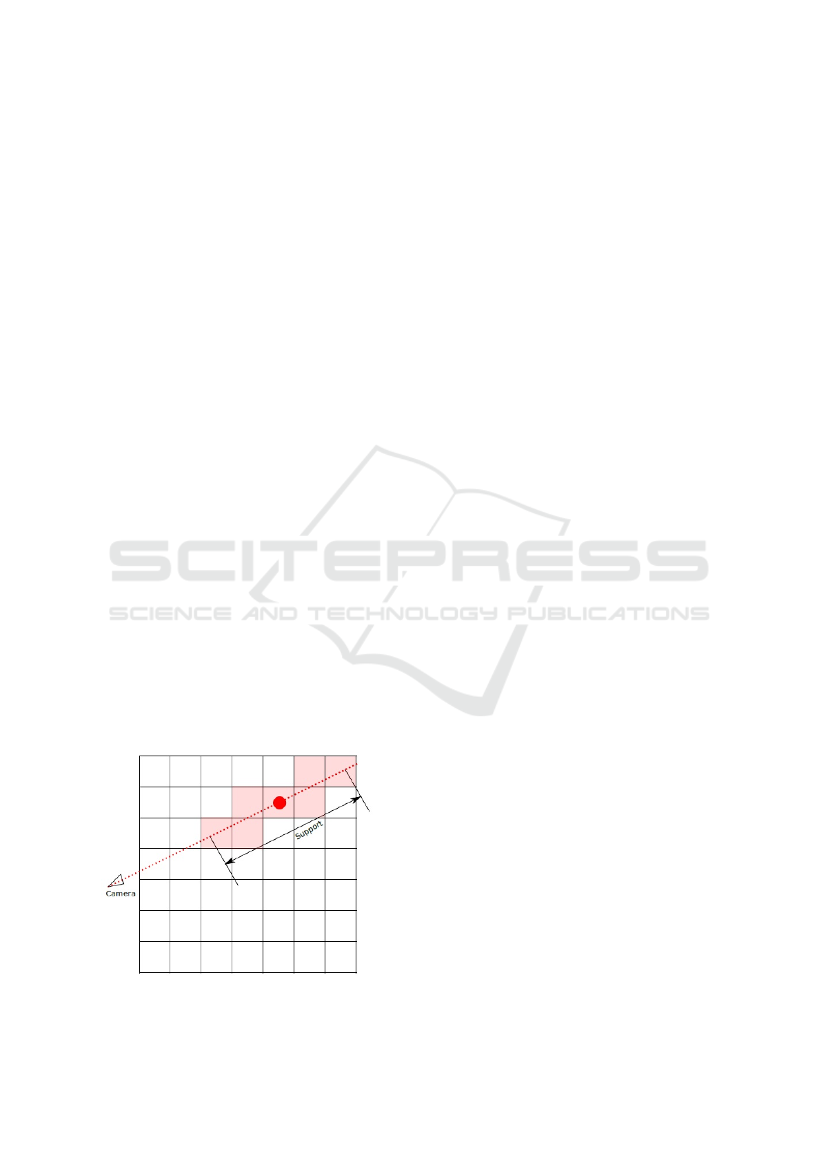
implicit surface. However our proposed scheme uses

only those voxels which lie along-the-ray from cam-

era center Cam

and a 3D sample position in world

space P

, this selection of voxels referred as SDF-

signal as shown in ﬁgure 1. In our implementation

we use linear Truncated Signed Distance Function

(TSDF) which ranges between [+1, ..., −1], which re-

sults in implicit representation having zero-crossing

at the given depth. These SDF-Signals are then used

directly in recursive fusion framework.

Since the main objective of proposed scheme is to

optimize depth fusion and enhance overall 3D recon-

struction, we incorporate ground truth camera poses

during fusion process. This assumption prevents all

Recursive Total Variation Filtering Based 3D Fusion

the problems related to failed tracking in SLAM and

ensures that optimization is focused on depth fusion.

4.2 Recursive TV 3D Fusion

Proposed scheme uses the recursive aspect of Least

Square Estimation (LSE) in which depth fusion is

achieved by solving the system of linear equation. As-

suming x ∈ R

is SDF signal containing current state

of system and y ∈ R

is SDF signal generated from

particular depth sample with n being the ray support

length in voxels. In order to fuse these two SDF sig-

nals using least squares we assume that transforma-

tion function between x and y is linear in nature. Thus,

least square estimate ˆx is that value of y that mini-

mizes the residual error

kAx + yk

(2)

In order to add inherent Total Variation ﬁltering based

regularization in proposed technique, we can take ad-

vantage by accessing the values in neighboring vox-

els. Hence minimization function for such regularized

recursive system can be re-written as

kAx + yk

+ λkg(x)k

(3)

Where λ is regularization parameter and g(x) is func-

tion which approximate the second order ﬁnite differ-

ence. Although the number of voxels in SDF signal

(referred compactly as Support in further description)

depends upon the scale of reconstruction and noise,

for explanation purpose we assume support n = 5

voxels. Assuming that v

k+1

= {a

, a

, ...a

} is a

SDF signal represented as a vector containing all the

voxels on a ray through a 3D sample (Figure 1) and a

represents the SDF values of these voxels before the

update the Equation 3 can be written as

kAx + yk

+ λkDv +Ck

(4)

Figure 1: SDF signal and selected voxels.

Actual derivation of D, C matrices and simpliﬁca-

tion of Equation 4 is beyond the scope of this paper

however detail steps can be found in the Appendix 7.

Next, the proposed technique is compactly referred to

as RFusion.

4.3 Update Algorithm

Algorithm 1 shows a simpliﬁed version of RFusion

which describes how the SDF signal is accessed and

updated. In actual implementation the algorithm was

implemented using threads to maximize the efﬁciency

and utilize the latest CPU architecture. We start our

fusion application by instantiating an object of data

structure proposed by (Funk and B

orner, 2016) in line

1. For each pixel(row, col) individual steps for fusion

algorithm are:

• calculation of 3D world coordinate P

at (row,

col), line 10

• getting RGB value at (row, col), line 11

• generating linear TSDF values (i.e. [+1, ..., −1])

depending upon the support, line 12

• reading current SDF value from voxels and creat-

ing SDF signal from W , line 13

• getting value of d and c matrices using method

describe in Appendix 7

• compute the new SDF signal y

from previous es-

timate ˆx

t−1

, line 15

• updating the W with latest estimate for particular

depth sample in line 16

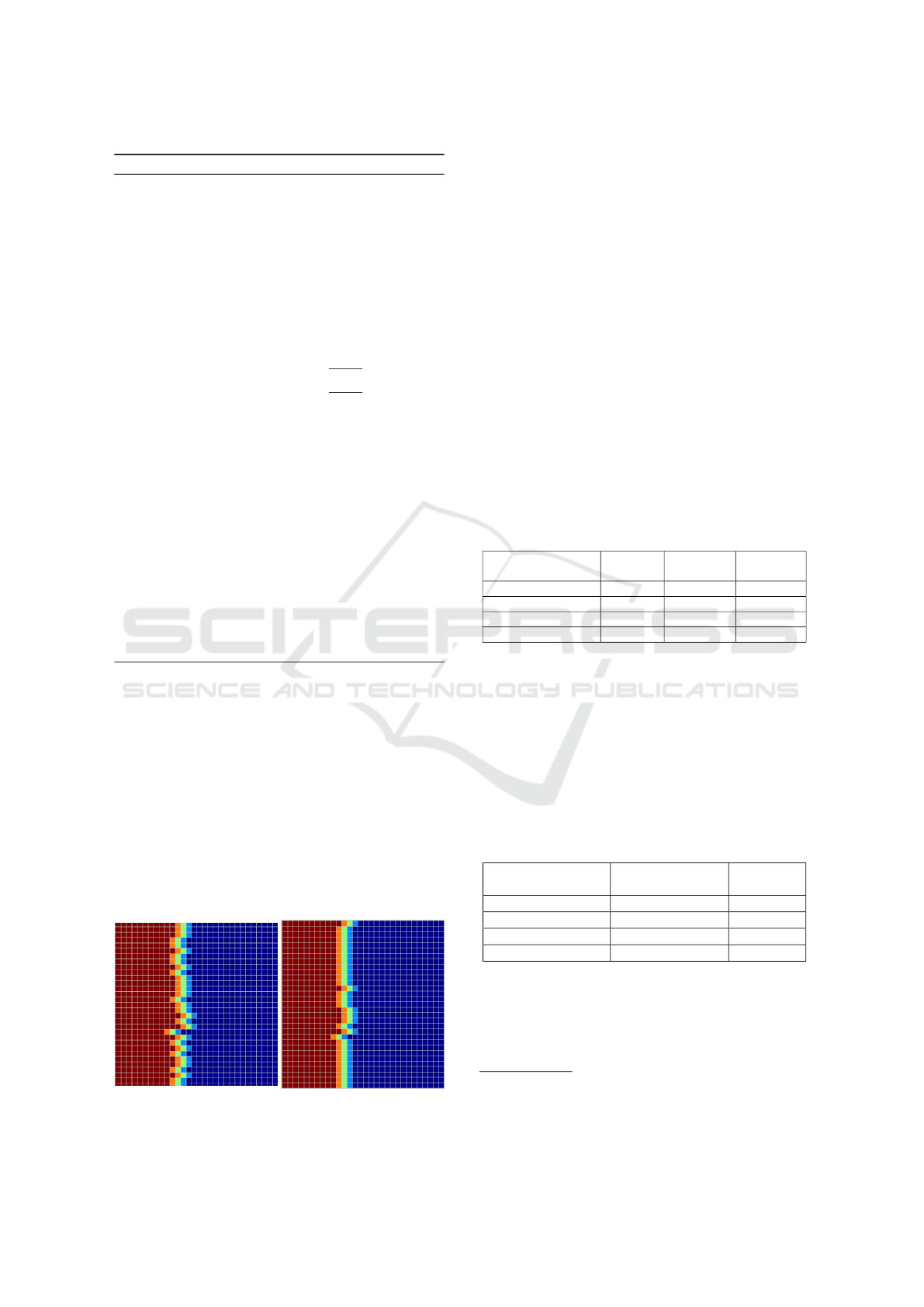
4.4 Effects of Regularization

In order to investigate and visualize the effects of

regularization parameter λ on noise suppression and

optimized depth fusion, we implemented 2D variant

of the proposed scheme. To avoid the effects of fu-

sion from regularization, single synthetic surface is

fused with itself. It was observed that TV ﬁltering

produced inherent smoothing effect on voxels at the

time of SDF signal fusion. This regularization effect

is demonstrated in Figure 2, where red cells repre-

sent positive values and blue cells represent negative

TSDF values.

5 EXPERIMENTS

5.1 ICL RGBD Dataset

In order to analyze the working of proposed scheme

we used synthetic RGBD dataset provided by ICL-

NUIM (Handa et al., 2014) which is considered to be

SIGMAP 2016 - International Conference on Signal Processing and Multimedia Applications

Algorithm 1: Simpliﬁed RFusion algorithm.

1: let W ← DataStructure (from (Funk and B

orner,

2016))

2: procedure FUSE

3: t ← currentFrame

4: I

← RGB image and Z

← Depth image

5: T

← Translation

6: R

← Rotation

7: support ← 5

8: for i = 0 to rows-1 do

9: for j = 0 to cols-1 do

10: P

← R







(x − c

)

Zt(x,y)

(y − c

)

Zt(x,y)

Zt(x, y)







+ T

11: color ← I

.getColor(i,j)

12: y

←getTSDF()

13: ˆx

t−1

← W.readVoxels(P

,support)

14: [d,c] ← W.getDC(x) (from eq. 20)

15: ˆx

← ˆx

t−1



φ(y

−λd

c)−(φ

φ+

λd

d) ˆx

t−1



(from eq. 13)

16: W .updateSystem( ˆx

,color)

17: end for

18: end for

19: t ← t + 1

20: end procedure

standard in depth fusion and 3D reconstruction eval-

uation. We have tested proposed scheme with and

without noise for thorough evaluation.

5.2 Evaluation

Since the dataset is synthetic in nature, it is possi-

ble to evaluate reconstructed model with actual model

afterwards. After necessary alignment and scaling,

for each vertex in the reconstructed model a clos-

est triangle is registered and perpendicular distance

is recorded. Five standard statistics (Mean, Median,

Figure 2: (left) illustrates an implicit surface with noise;

(right) demonstrates the effects of regularization parameter.

Standard Deviation, Min and Max etc) can be com-

puted from the recorded distance as suggested by

(Handa et al., 2014).

However we will analyze the performance of each

framework with mean and standard deviation of stan-

dard statistics.

Candidates for quantitative comparison are fol-

lowing fusion frameworks:

1. Fast Fusion (Steinbruecker et al., 2014)

2. RFusion

3. InﬁniTAM

ahler et al., 2015)

It is worth mentioning that similar to proposed tech-

nique, ground truth camera poses ware used instead

of tracking to avoid any biased evaluation. Figure 3

illustrates the reconstruction with our proposed tech-

nique vs the reconstruction from FastFusion. It was

observed that RFusion was able to fuse minute details

of model (such as lamp pole, leaves of plant etc) into

single connected mesh however FastFusion generated

multiple inconsistent meshes.

Table 1: Comparision of absolute surface error (in meters).

Dataset

Method

RFusion FastFusion InﬁniTAM

LR0 0.003045 0.011895 0.008900

LR1 0.002947 0.011204 0.002900

LR2 0.003183 0.006634 0.008800

LR3 0.002978 0.018180 0.041000

During experimentation phase it was observed

that RFusion gives improved performance compared

to state of art fusion techniques and achieved 4-5

frames per second on pure CPU based implementa-

tion.

System used for experimentation has the follow-

ing speciﬁcations: Intel Core i7-4790, 8GB RAM

with Windows 7 (64-bit) OS.

Table 2: Comparision of absolute surface error on noisy

dataset (in meters).

Dataset

Method

RFusion (λ = 0.3) FastFusion

LR0 0.01336 0.05672

LR1 0.01416 0.07523

LR2 0.01979 0.07082

LR3 0.02090 0.06643

Since we ware not able to modify the working of Inﬁni-

TAM with ICL-NUIM dataset we are using the Mean val-

ues published in (K

ahler et al., 2015) for this dataset

Recursive Total Variation Filtering Based 3D Fusion

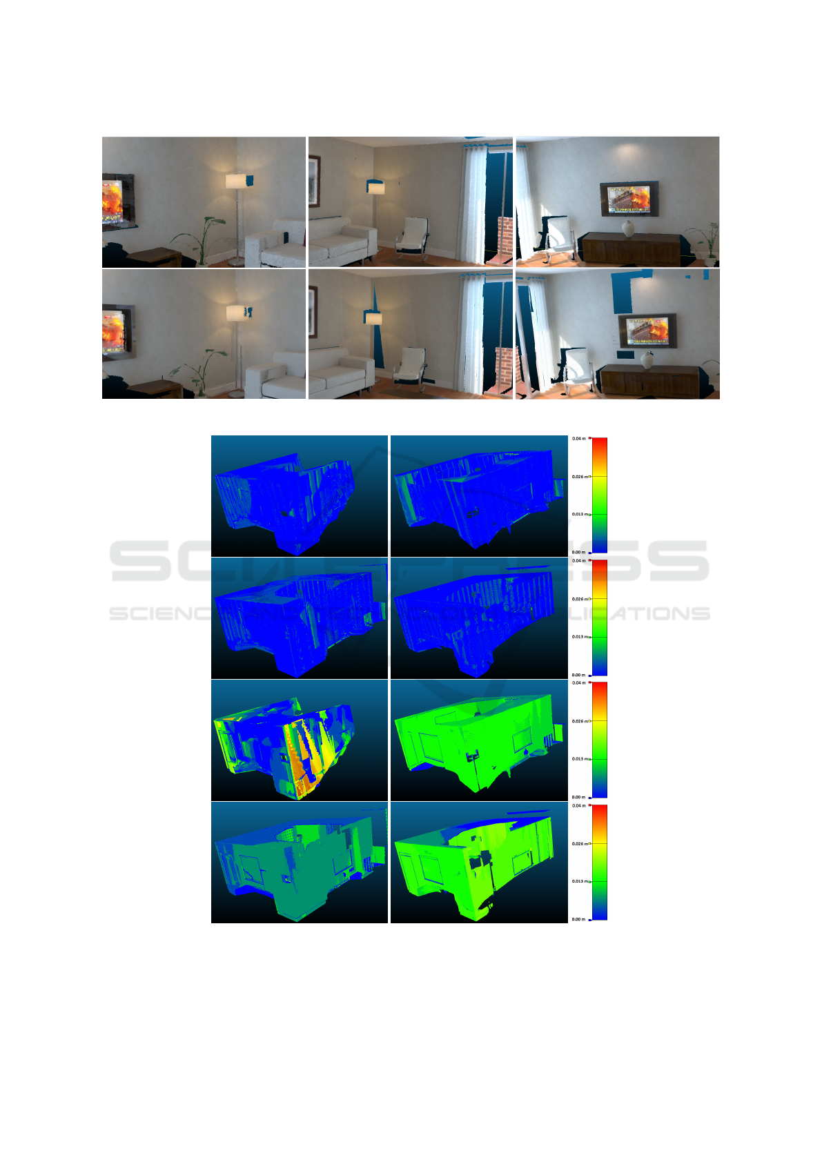
Figure 3: Screenshots from reconstructed model with RFusion (upper row) and FastFusion (bottom row).

Figure 4: Color coded errormaps from RFusion (Upper 2 rows) vs FastFusion (Bottom 2 rows) along with absolute color scale

used to genarate errormaps.

SIGMAP 2016 - International Conference on Signal Processing and Multimedia Applications

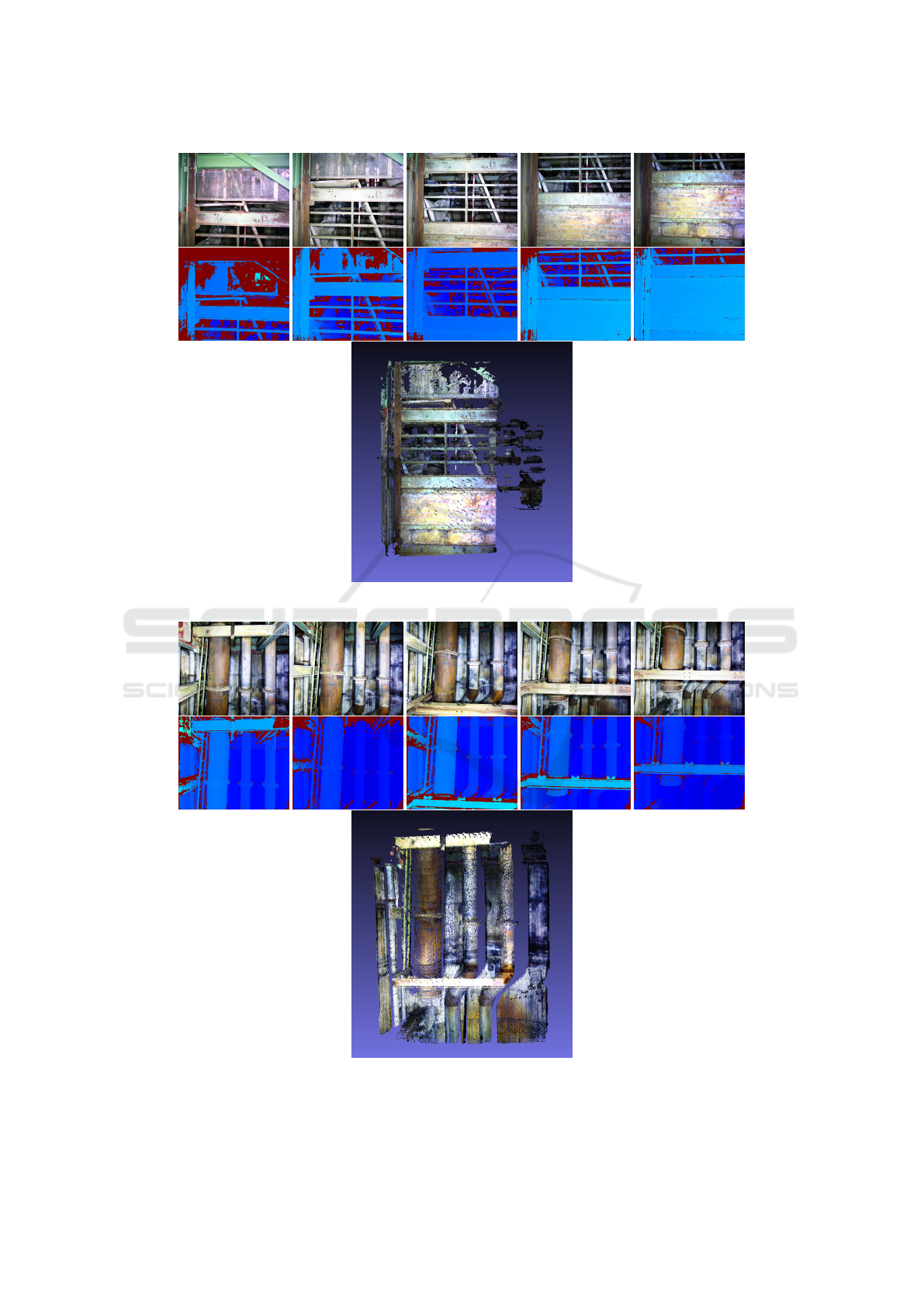
Figure 5: RGB images (upper row), depth images (second row) and reconstructed 3D model (last row).

Figure 6: RGB images (upper row), depth images (second row) and reconstructed 3D model (last row).

Recursive Total Variation Filtering Based 3D Fusion

6 EXPERIMENTATION RESULTS

FROM IPS DATA

In order to evaluate the working of proposed system

with real data, we used dataset captured from stereo

camera based IPS (Baumbach and Zuev, 2014). Since

the data is real in nature, it is not feasable to evaluate

the absolute surface error of reconstructed model and

actual environment. Therefore Screenshots of such

reconstruction are illustrated in ﬁgure 5 and 6 for vi-

sual inspection and evaluation.

7 CONCLUSION AND OUTLOOK

In this paper, we presented a novel approach to ad-

dress the challenges related to 3D depth fusion and

reconstruction with the use of L2 regularization based

recursive fusion framework. We demonstrated that

the proposed system has potential of reducing noise

along with capability of incremental 3D depth fusion.

At current state, implementation of proposed scheme

is purely threads based CPU processing, however fur-

ther implementation is required to extend the frame-

work to utilize latest GPU computation power along

with CPU processing. Furthermore, since the system

handles noise inherently, it would be interesting to in-

tegrate planar simpliﬁcation techniques for improved

3D reconstruction in future research exploration.

REFERENCES

(2014). ATAP Project Tango Googl. http://www.google.

com/atap/projecttango/. Accessed: 2015-11-22.

Baumbach, D. G. D. and Zuev, S. (2014). Stereo-Vision-

Aided Inertial Navigation for Unknown Indoor and

Outdoor Environments. In Proceedings of the Interna-

tional Conference on Indoor Positioning and Indoor

Navigation (IPIN), 2014 . IEEE.

Chen, J., Bautembach, D., and Izadi, S. (2013). Scalable

real-time volumetric surface reconstruction. ACM

Trans. Graph., 32(4):113:1–113:16.

Christopher Urmson et. al (2008). Autonomous driving in

urban environments: Boss and the urban challenge.

Journal of Field Robotics Special Issue on the 2007

DARPA Urban Challenge, Part I, 25(8):425–466.

Curless, B. and Levoy, M. (1996). A volumetric method for

building complex models from range images. In Pro-

ceedings of the 23rd Annual Conference on Computer

Graphics and Interactive Techniques, SIGGRAPH

’96, pages 303–312, New York, NY, USA. ACM.

Dahlkamp, H., Kaehler, A., Stavens, D., Thrun, S., and

Bradski, G. (2006). Self-supervised monocular road

detection in desert terrain. In Proceedings of Robotics:

Science and Systems, Philadelphia, USA.

Funk, E. and B

orner, A. (2016). Inﬁnite 3d modelling vol-

umes. In VISAPP 2016.

Handa, A., Whelan, T., McDonald, J., and Davison, A. J.

(2014). A benchmark for rgb-d visual odometry, 3d

reconstruction and slam. In Robotics and Automa-

tion (ICRA), 2014 IEEE International Conference on,

pages 1524–1531. IEEE.

Hicks, S. L., Wilson, I., Muhammed, L., Worsfold, J.,

Downes, S. M., and Kennard, C. (2013). A depth-

based head-mounted visual display to aid naviga-

tion in partially sighted individuals. PLoS ONE,

8(7):e67695.

Izadi, S., Kim, D., Hilliges, O., Molyneaux, D., Newcombe,

R., Kohli, P., Shotton, J., Hodges, S., Freeman, D.,

Davison, A., and Fitzgibbon, A. (2011). Kinectfu-

sion: Real-time 3d reconstruction and interaction us-

ing a moving depth camera. In ACM Symposium on

User Interface Software and Technology. ACM.

ahler, O., Prisacariu, V. A., Ren, C. Y., Sun, X., Torr,

P. H. S., and Murray, D. W. (2015). Very High

Frame Rate Volumetric Integration of Depth Images

on Mobile Device. IEEE Transactions on Visualiza-

tion and Computer Graphics (Proceedings Interna-

tional Symposium on Mixed and Augmented Reality

2015, 22(11).

Newcombe, R. A., Lovegrove, S. J., and Davison, A. J.

(2011). Dtam: Dense tracking and mapping in real-

time. In Proceedings of the 2011 International Con-

ference on Computer Vision, ICCV ’11, pages 2320–

2327, Washington, DC, USA. IEEE Computer Soci-

ety.

Rudin, L. I., Osher, S., and Fatemi, E. (1992). Nonlinear to-

tal variation based noise removal algorithms. Physica

D: Nonlinear Phenomena, 60(14):259 – 268.

Steinbruecker, F., Sturm, J., and Cremers, D. (2014). Volu-

metric 3d mapping in real-time on a cpu. In Int. Conf.

on Robotics and Automation, Hongkong, China.

uhmer, J., Gumhold, S., and Cremers, D. (2010). Real-

time dense geometry from a handheld camera. In Pat-

tern Recognition (Proc. DAGM), pages 11–20, Darm-

stadt, Germany.

Taneja, A., Ballan, L., and Pollefeys, M. (2013). City-scale

change detection in cadastral 3d models using images.

In Computer Vision and Pattern Recognition (CVPR),

Portland.

APPENDIX

Derivation of RFusion

In this section we derive the equations of RFusion,

for the sake of better readability we will simplify the

equations for 2D fusion system rather than 3D fusion

system. Assuming n = support of SDF signal, ˆx is

estimated state of system for particular 3D voxel and

y = new TSDF signal. Then such system can easily be

SIGMAP 2016 - International Conference on Signal Processing and Multimedia Applications

describe by the following equation.

y = φ ˆx

ˆx = (φ

φ)φ

y (5)

In order to integrate the true aspect of second order

ﬁnite difference it is assumed that

Y = Y − λD

C (6)

Since equation 5 is only valid if we have single in-

put SDF signal, we assume that we have multiple

SDF signals, Then we can extend equation 5 for batch

based least square system as follows







0∗1

0∗2

...

0∗n

1∗1

...

m∗n













1 0 0 0 0

0 1 0 0 0

...

0 0 0 0 1

1 0 0 0 0

...

0 0 0 0 1







ˆx

where m is the number of SDF signals about to be

merged

Y = Φx

x = (Φ

Φ)Φ

The regularized variant of batch-based system can be

re-written as

ˆx =



Φ + λD



Y (7)

where λ is a regularization parameter. In order to con-

vert batch based system to recursive system we as-

sume that Φ,Y and D follow recursive succession

k+1





k+1



ˆy



andD

k+1





Equation 7 for k + 1 instance can be written as

ˆx

k+1



k+1

+ λD

k+1



−1

k+1

(8)

For better readability we use substitution of P

−1

k+1

from

equation (15) and using the recursive versions of Φ

and Y we get

ˆx

k+1

= P

k+1

−1

k+1

ˆx

k+1

= Φ

k+1

(9)

Similarly for k

instance

= P

−1

ˆx

(10)

Resuming from equation (9) we get

ˆx

k+1

= P

k+1



+ φ

ˆy

k+1



By using the value of Φ

from equation (10) we

get

ˆx

k+1

= P

k+1



−1

ˆx

+ φ

ˆy

k+1



By using the value of P

−1

from equation (16) we

get

ˆx

k+1

= P

k+1



−1

k+1

− (φ

φ + λd



ˆx

+ φ

ˆy

k+1





k+1

−1

k+1

− P

k+1

(φ

φ + λd



ˆx

+ P

k+1

ˆy

k+1

= P

k+1

−1

k+1

ˆx

− P

k+1

(φ

φ + λd

d) ˆx

+ P

k+1

ˆy

k+1

= ˆx

− P

k+1



φ + λd



ˆx

+ P

k+1

ˆy

k+1

ˆx

k+1

= ˆx

+ P

k+1



φ ˆy

k+1

− (φ

φ + λd

d) ˆx



(11)

by using the assumption from equation (6) we can fur-

ther assume that

ˆy

k+1

= y

k+1

− λd

Hence ﬁnal equation (11) for RFusion will be-

come

ˆx

k+1

= ˆx

+ P

k+1



φ(y

k+1

− λd

c) − (φ

φ + λd

d) ˆx



(12)

From the fundamental regularized LSE equation

ˆx

k+1



Φ + λD



−1

Let P



Φ + λD



−1

(13)

−1



Φ + λD



(14)

For the recursive part we can extend the Φ and D

matrices as follows

k+1





and D

k+1





Recursive Total Variation Filtering Based 3D Fusion

Then equation (14) will become

k+1









+ λ











−1

k+1



Φ + φ

φ + λD

D + λd



−1

k+1



(Φ

Φ + λD

D) + φ

φ + λd



−1

k+1



−1

+ (φ

φ + λd



−1

(15)

−1

k+1

= P

−1

+ (φ

φ + λd

−1

= P

−1

k+1

− (φ

φ + λd

d) (16)

k+1



−1



φ I





λd

 

−1

For simplicity assuming

B =



φ I



and C =



λd



we get

k+1



−1

+ BC



−1

Using matrix inversion lemma

(A + BC)

−1

= A

−1

− A

−1

B(I +CA

−1

k+1

= P

− P

B(I +CP

−1

(17)

Formulation of D Matrix

Since we are dealing with elements in a 2D matrix

each cell and respective neighboring cells can be ac-

cessed by their respective spatial information (i.e. row

and column values in case of 2D), however actual im-

plementation of proposed technique is carried to han-

dle 3D depth fusion. For each voxel value a

(where

0>k>support) in vector SDF signal v, assuming that

i and j are index values of row and column respec-

tively for accessing a

in equation (15), ﬁnite differ-

ence in vector form can be written as

∇a







∇













∇













a(i − 1, j) − 2a(i, j) + a(i + 1, j)

a(i, j − 1) − 2a(i, j) + a(i, j + 1)

a(i+1, j+1)−a(i+1, j)−a(i, j+1)+2a(i, j)−a(i−1, j)−a(i, j−1)+a(i−1, j−1)







(18)

Elements of equation (15) can be separated depend-

ing upon if the elements are in the incident ray which

is currently being fused or in neighboring cell. The

separated elements can then be written using multiple

matrix form as

∇a

= D

v +C

(19)

where







−2 1 0 ... 0

−2 0 0 ... 0

1 0.5 0 ... 0













a(i − 1, j)

a(i, j − 1) + a(i, j + 1)

a(i+1, j+1)−a(i+1, j)−a(i−1, j)−a(i, j−1)+a(i+1, j+1)







and C

matrix in equation (19) are only valid

for a

(where k = 1). However by using the same

method, composite D and C matrix can be formulated

and written as

∇v =







∇a

...

∇a













...







v +







...







∇v = Dv +C (20)

Matrix C from equation (20) is used in the later stages

of RFusion to incorporate the integrated smoothing.

Values of D and C matrices are calculated on run time,

hence elements depend upon the angle of ray, size of SDF

width etc.

SIGMAP 2016 - International Conference on Signal Processing and Multimedia Applications