
Lithium-ion Batteries Aging Motinoring Througth Open Circuit
Voltage (OCV) Curve Modelling and Adjustment
Loic Lavigne
1
, Jocelyn Sabatier
1
, Junior Mbala Francisco
2
,
Franck Guillemard
2
and Agneiszka Noury
2
1
IMS Laboratory, UMR 5218 CNRS, Bordeaux University, 351 Cours de la Libération, 33405 Talence, France
2
PSA Peugeot Citroën ,2 Route de Gisy, 78943 Vélizy-Villacoublay, France
Keywords: Lithium-ion Cell, Open Circuit Voltage (OCV) Curve Adjustment, Battery Aging Monitoring.
Abstract: This paper is a contribution to lithium-ion batteries modeling tacking into account aging effects. It first
analyses the impact of aging on electrode stoichiometry and then on lithium-ion cell Open Circuit Voltage
(OCV) curve. Through some hypotheses and an appropriate definition of the cell state of charge, it shows
that each electrode equilibrium potential, but also the whole cell equilibrium potential can be modelled by a
polynomial that requires only one adjustment parameter during aging. An adjustment algorithm, based on
the idea that for two fixed OCVs, the state of charge between these two equilibrium states is unique for a
given aging level, is then proposed. Its efficiency is evaluated on a battery pack constituted of four cells.
This adjustment parameter can thus be viewed as a State Of Health (SOH) or aging indicator.
1 INTRODUCTION
Due to their high energy and power densities
compared to other existing technologies, Li-ion
batteries are increasingly used as energy storage
system in mobile applications (Armand and
Tarascon, 2008). The onboard Li-ion battery packs
have to work together with reliable battery
management systems (BMS) to ensure their optimal
and safe use (Liaw et al, 2010). Among the tasks
ensured by the BMS, State-Of-Charge (SOC)
estimation is of an extreme importance. The energy
management strategies in hybrid vehicles, for
instance, rely on the accurate knowledge of the
SOC, the latter being an indicator of available
energy. SOC estimation methods commonly used
impose a characterization of the Open Circuit
Voltage (OCV) curve (through a polynomial, a look-
up table, …) as they use :
- either a direct OCV curve inversion methods (if
the application permits cells steady state voltage
measurement) (Lee et al, 2008),
- or cells models based methods (Plett, 2004),
(Kim, 2010), (Sabatier et al, 2014), (Francisco et
al, 2014), (Sabatier et al, 2015).
As OCV is closely related to SOC, the SOC
estimators require an accurate OCV model (Piller et
al, 2001), (Santhanagopalan and White, 2006).
However, at battery aging, the OCV curve of
each cell changes as OCV reflect battery aging and
performance degradation (Roscher et al, 2011). The
impact of aging on cell equilibrium voltage is
analyzed in (Schmidt and al, 2013). This change
distorts the estimator if nothing is done to adjust the
curve law. Aging correction can be thus
implemented as done in (Cheng et al, 2015). But this
class of methods does not take into account the
underlying physical phenomenon of lithium-ion
intercalation process. This knowledge makes
possible analytical descriptions of the OCV curve
and then permits the implementation of accurate
estimation methods for both SOC and State of
Health (SOH). Some of these methods are known in
the literature as incremental capacity analysis (ICA)
technique (Dubarry and Liaw, 2009) or the
differential voltage analysis (DVA) (Honkuraa et al,
2008).
Most of the analytical descriptions for OCV
curve available in the literature involve a large
number of parameter (Hu et al, 2011), (Weng et al,
2014) that all must be adjusted as battery aging. This
imposes to implement complex and resources
consuming on-board iterative optimization
Lavigne, L., Sabatier, J., Francisco, J., Guillemard, F. and Noury, A.
Lithium-ion Batteries Aging Motinoring Througth Open Circuit Voltage (OCV) Curve Modelling and Adjustment.
DOI: 10.5220/0005961400570067
In Proceedings of the 13th International Conference on Informatics in Control, Automation and Robotics (ICINCO 2016) - Volume 1, pages 57-67
ISBN: 978-989-758-198-4
Copyright
c
2016 by SCITEPRESS – Science and Technology Publications, Lda. All rights reserved
57

algorithms.
In this paper, a new polynomial parametrization
for OCV curve is proposed. As ageing of lithium-ion
cell, only one parameter must be adjusted to ensure
an accurate fitting of the OCV curve by the
polynomial. Such a parametrization results in an
analysis of the cell using "communicating vessels”
idea introduced in (Schmidt and al, 2013). If each
electrode equilibrium voltages at the unused state is
modelled as in (Karthikeyan et al, 2008),
introduction of some simplifying hypothesis permits
to show that the OCV curve can be modelled by a
polynomial that requires only one adjustment
parameter during aging. An adjustment algorithm,
based on the idea that for two fixed OCVs, the state
of charge between these two equilibrium state is
unique for a given aging level, is then proposed. Its
efficiency is evaluated on a battery pack constituted
of four cells.
2 PARAMETRIZATION OF A
LITHIUM-ION CELL OCV
2.1 Notations and Electrode
Equilibrium Potential Definition
It is supposed in the sequel that subscript p and n are
used to denote respectively the positive and the
negative electrode of a lithium-ion cell. Electrodes
stoichiometry x
i
, i{p, n} (Bard et al., 2008) are
defined as the ratio of the inserted lithium quantities
Q
i
over the maximal theoretical quantities that can
be inserted Q
i,max
:
tQ
tQ
tx
i
i
i
max,
.
(1)
If T denotes the temperature, cell OCV can be
defined using the equilibrium potentials of the two
electrodes, by:
TxETxETE
nnpp
,,
,
(2)
positive electrode equilibrium potential, denoted
TxE
pp
,
, and negative electrode equilibrium
potential, denoted
TxE
nn
,
, being respectively
defined by:
iINTiNernstii
xVTxVTxE ,,
pni ,
.
(3)
Using standard potential
0
i
E
, Nernst potential
TxV
iNernst
,
, is defined by the relation
i
i
iiNernst
x
x
F
RT
ETxV
1
ln,
0
pni ,
.
(4)
In the previous relation, R denotes the universal
gas constant (R = 8.314 472 J K
−1
mol
−1
) and F is the
Faraday constant (F=96485.33°C mol
−1
). Among the
models available in the literature for
iINT
xV
,
Redlich-Kister model given by the following
relation is used in the sequel (Karthikeyan, Sikha,
and White 2008) with
pni ,
:
k
i
ii
k
i
K
k
kiiINT
x
xkx
xAxV
i
1
1
0
,
12
12
12
.
(5)
It is the expression of V
INT
(for non-ideal
interaction), that gives the closest experimental
measures fitting as shown in Figure 1, comparing to
several other equilibrium potential laws
(Karthikeyan, Sikha, and White 2008).
Remark 1 - According to relation (21) and (22) in
(Karthikeyan, Sikha, and White 2008), note that a
linear dependence to temperature can be introduced
in coefficients
ki
A
,
to take into account temperature
variations:
TaTA
kiki ,,
(
ki
a
,
being an additional
parameter for temperature dependence such as for
0,,
TaA
kiki
for parameters
ki
A
,
in relation (5) and
for a reference temperature T
0
).
Figure 1: Comparison of various equilibrium electrode
potentials laws for experimental data fitting (Karthikeyan,
Sikha, and White 2008).
2.2 Polynomial Approximations of
Electrode Equilibrium Potentials
The goal now is to make simplifying assumptions in
order to obtain polynomial expressions for
electrodes equilibrium potentials.
Given that
ICINCO 2016 - 13th International Conference on Informatics in Control, Automation and Robotics
58

)1(1ln1ln
1
ln
ii
i
i
xx
x
x
pni ,
(6)
expansion of
xx1ln
on
1,0x
is given by:
0
1
1
0
1
1
1
1
1
1
ln
k
k
i
k
k
k
i
i
i
k
x
k
x
x
x
(7)
with
pni ,
and permits the following
approximation, denoted
TxV
iNernst
,
~
, for relation
(4):
111
0
0
11
1
1
,
k
i
k
i
k
N
k
iiNernst
xx
kF
RT
ETxV
i
LN
(8)
Thus, for a large enough N
i
LN
, the function
FxxRT
ii
1ln
can be reduced to a
polynomial. By way of illustration, Figure 2 shows
that the approximation error
TxVTxV
iNernstiNernst
,
~
,
remains minor and
limited to a few millivolts and also shows a low
impact of temperature T.
Thus, using relation (8) and through expansion
of relation (5), electrode equilibrium potentials in
relation (2) can be written in polynomial form:
i
N
k
k
ikii
xAE
0
,
pni ,
(9)
with
i
LNii
NKN ;max
.
(10)
where coefficients
ki
A
,
are combinations of
coefficients
ki
A
,
of relation (5).
As shown in the application section, temperature
has a low impact on coefficients
ki
A
,
but according
to remark 1, temperature dependence can be
introduced in coefficients
ki
A
,
and thus relation (9)
can be rewritten as:
i
N
k
k
ikiiii
xTaTaaE
1
,
10
pni ,
.
(11)
2.3 Ageing Effects on Electrodes
Stoichiometry
From relation (9), cell OCV depends on:
Figure 2: Approximation error between
TxVTxV
iNernstiNernst
,
~
,
for various values of N
i
LN
(a) and impact of the temperature on
TxV
iNernst
,
with
0
0
i
E
(b).
- parameters
0
i
E
,
ki
A
,
and more weakly on the
temperature T;
- electrodes stoichiometries x
i
which themselves
depends on the amount of inserted lithium
i
Q
and
the maximal theoretical capacity
max,i
Q
according
to relation (1).
In agreement with the authors of (Karthikeyan et
al. 2008), the following assumption is made on
coefficients
ki
A
,
.
Hypothesis 1
For a constant temperature, coefficients
ki
A
,
of
Redlich-Kister model are supposed constants as
intrinsic to the electrode electrochemistry
∎
As a consequence, coefficients
ki
A
,
are not
affected by the cell aging. Aging is then necessarily
passed on electrodes stoichiometry
p
x
and
n
x
.
0 0.1 0.2 0.3 0.4 0.5 0.6 0.7 0.8 0.9 1
-0.06
-0.04
-0.02
0
0.02
0.04
0.06
x
i
V
Nernst
-V
~
Nernst
(V)
N
i
LN
=10
N
i
LN
=20
N
i
LN
=30
0 0.1 0.2 0.3 0.4 0.5 0.6 0.7 0.8 0.9 1
-0.2
-0.15
-0.1
-0.05
0
0.05
0.1
0.15
x
i
V
Nernst
(V) for E
i
0
=0
T=20°C
T=-10°C
T=50°C
(a)
(b)
Lithium-ion Batteries Aging Motinoring Througth Open Circuit Voltage (OCV) Curve Modelling and Adjustment
59

Specifically, it is then expected that the only aging
reactions impacting the cell OCV are those resulting
in at least one of the following effects:
- a change in the electrode geometry, (eg
formation of dendritic deposits (Arora et al. 1998))
this change impacting the cell theoretical maximum
capacity
max,i
Q
and thus the stoichiometry
tx
i
linked to the amount of charge
tQ
i
in electrode i;
- a loss
Li
cycling ions (ion consumption in
aging reactions).
Since the cell OCV characterizes a cell at rest,
charge transfer equations can be ignored in the
following developments. For the analysis of
Li
cycling ions concentration, the cell will be
represented by two communicating tanks as in (Po et
al. 2007).
In the previous equations, the OCV is expressed
according to electrode stoichiometries. We now
establish the link between the electrode
stoichiometries and the SOC (estimated in practice).
This last one is defined by the relation:
ref
dispo
Q
Q
SOC
(12)
where Q
dispo
is the possible capacity extractible of
the cell. In usual definition of SOC, Q
ref
is the cell
maximum capacity which varies with aging cells.
This is a problem if OCV adjustment during aging
requires SOC measures, as SOC definition requires
the cell real capacity knowledge which is precisely
to identify. To treat this problem, the Q
ref
uncertainty
during aging is eliminated by adopting the following
definition:
Definition 1
tE
E
ref
tConsQIif
EEif
tSOC
%100
tan0
%100
%100
.
(13)
Figure 3: Link between the electrodes stoichiometry and
the SOC.
This definition imposes
- a SOC equal to 100% when OCV is maximum
and equal to E
100%
(for example 4V) for all cells
ageing.
- a SOC equal to 0% after discharge, starting to
E = E
100%
, and a fixed Q
ref
. The Q
ref
choice is not
important and is determined by the user. In practice
the reference capacity is usually fixed to the nominal
capacity (Q
ref
= Q
nom
). Definition 1 is illustrated in
Figure 3.
For an electrode i (i{n, p}), and as illustrated
by Figure 4, the available capacity can be defined
by:
0,iiav
QQQ
(14)
where Q
i,0
is the capacity in the electrode at SOC =
0, then
max,0,0, iii
QQx
is the electrode
stoichiometry for SOC = 0%.
Figure 4: Available capacity definition for an electrode.
From relation (1) and previous analysis:
0
0,
max,
0,
max,
i
i
i
i
i
i
x
tQ
tQ
tQ
tQ
tx
(15)
then
0,
max,
0,
max,
0,
i
i
dispo
i
i
ii
i
x
tQ
tQ
x
tQ
tQtQ
tx
(16)
or
0,
max,
i
refi
disporef
i
x
tQtQ
tQtQ
tx
(17)
and finally
0,
max,
)(
i
i
ref
i
xtSOC
tQ
tQ
tx
.
(18)
Then, for SOC = 100%, the following equation is
ICINCO 2016 - 13th International Conference on Informatics in Control, Automation and Robotics
60

verified
tQtQtxtx
irefii max,0,100,
.
The previous analysis shows that the electrode
stoichiometries are proportional to the SOC and can
be written:
0,0,100,
0,0,100,
nnnn
pppp
xSOCxxtx
xSOCxxtx
.
(19)
Let us consider a given state of charge
SOC. The
corresponding OCV is varying with cell aging,
excepted for the point
SOC =100% (according to
definition 1). For the positive electrode, this change
modifies the parameter
x
p,0
which is then depending
of cell aging (
x
p,0
x
p,0
(age)). The parameter
p
(age) is then introduced such as:
agextSOCage
Q
Q
tx
pp
init
p
ref
p 0,
max,
(20)
or with a more compact form :
agetSOCagetx
ppp
,
(21)
where
agexage
age
Q
Q
age
pp
p
init
p
ref
p
0,
max,
.
(22)
The same equation holds for the negative electrode
with parameters
age
n
and
age
n
:
agetSOCagetx
nnn
.
(23)
2.4 Open Circuit Voltage
Parametrization with Knowledges
of Each Cell Equilibrium Potential
In this section, equilibrium potentials E
p
and E
n
, and
then coefficients
kp
A
,
and
kn
A
,
are supposed
known. From relations (21) and (23), the equilibrium
potentials
E
p
and E
n
given by relation (9) can be
expressed as a function of cell ageing with the 4
parameters
age
p
,
age
p
,
age
n
and
age
n
, and thus relation (2) becomes:
,
0
,
0
p
n
N
k
pp
pk
k
N
k
nn
nk
k
EA ageSOC age
A age SOC age
.
(24)
The OCV adjustment problem after ageing
consists in the identification of these 4 parameters.
This adjustment can for instance, be realized with a
set of
M measures
Mj
jj
ESOC
;1
;
through
minimization of criteria:
2
1
1
M
jpp p
j
nn n
E E age SOC age
J
M
E age SOC age
,
(25)
with the constraint:
n
p
N
k
k
nnkn
N
k
k
ppkp
ageageA
ageageAE
0
,
0
,%100
:
C
.
(26)
As the SOC definition given by relation (13)
imposes a fixed Q
ref
capacity, estimation of
np
;
supplies maximum capacities estimations
max,p
Q
and
max,n
Q
.
2.5 Open Circuit Voltage
Parametrization without
Knowledge of Each Cell
Equilibrium Potential
When equilibrium potentials E
p
and E
n
are not
known (practical case),
kp
A
,
and
kn
A
,
coefficients
become unknowns. The only OCV curve available is
an experimental measure of this one obtained from
the interpolation of a set of OCV measures with
large SOC variations. This OCV curve will be noted
OCVC
init
. A study of different OCV measure
technics is given in (Petzl and Danzer, 2013).
Measures in charge and discharge are used to
determine the OCV curve. An average curve
obtained with a charge curve and a discharge curve
seems to be the best compromise because of
hysteresis effects (Roscher et al. 2011). OCV curves
(OCVC
init
) used in the following are determined for
discharge measures (see Figure 5).
Figure 5: OCVCinit identification with OCV measures.
The curve OCVC
init
obtained with polynomial
Lithium-ion Batteries Aging Motinoring Througth Open Circuit Voltage (OCV) Curve Modelling and Adjustment
61

interpolation at start time, has the following
structure:
N
k
kinit
kinit
SOCDE
0
.
(27)
To prove that aging impact on OCV can be
expressed like in relation (24), the link between the
two electrodes stoichiometries x
p
and x
n
is now
established.
In (Pop et al. 2007), a cell is represented for two
communicating tanks according to figure 6.
Figure 6: Cell Li-ion simplified scheme.
Figure 6 permits to write the following equation:
CstQQ
np
,
(28)
where by dividing by
max,p
Q
:
'
max,max,
Cst
Q
Q
Q
Q
p
n
p
p
(29)
and thus
'
max,
max,
max,
max,
max,
Cstx
Q
Q
x
Q
Q
Q
Q
x
n
p
n
p
p
n
n
n
p
.
(30)
Relation (30) shows that a linear equation can
connect the electrode stoichiometries x
p
and x
n
as:
pnpp
dxcx
(31)
or
npnn
dxcx
.
(32)
Then relation (2) becomes:
n
p
N
k
k
npnkn
N
k
k
pkp
dxcAxAE
0
,
0
,
.
(33)
Expansion of terms in the second sum permits a
new relation:
N
k
k
pk
NN
k
k
pk
xDxDE
np
0
,max
0
.
(34)
Coefficients
D
k
are combinations of coefficients
kp
A
,
,
kn
A
,
,
n
c
and
n
d
. The ageing impact on the
OCV, can then be introduced by relation (21), thus
leading to:
N
k
k
ppk
agetSOCageDE
0
.
(35)
Remark 2 - According to relation (11) in relation
(33), temperature dependence can be introduced in
relation (35), leading to
N
k
k
ppk
agetSOCageTd
TddE
1
10
(36)
From relation (35), the OCV adjustment problem
after ageing consists in the identification of only the
two parameters
p
and
p
. This identification can,
for instance, be realized with a set of
M measures
Mj
jj
ESOC
;1
;
through minimization of
criterion:
2
1
1
M
j
ppj
ageSOCageEE
M
J
.
(37)
with constraint:
N
k
k
ppk
ageageDE
0
%100
:
C
.
(38)
2.6 Experimental Validation
To experimentally validate the relation (35), several
OCV curves stemming from accelerated aging
process (described in section 3.1) are now identified
by assuming that the OCV after aging is given by:
N
k
k
k
ageSOCageDE
0
.
(39)
Search for
and
parameters is performed
manually. A wide range of values for
and are
used. For each pair (
,
), the following criterion is
evaluated:
ICINCO 2016 - 13th International Conference on Informatics in Control, Automation and Robotics
62
2
3
,
1
,
,, ,
mesures j
test
j
k mesures j
E
J
EDSOC
.
(40)
The three couples of measures
jmesuresjmesures
ESOC
,,
;
are derived from a charge
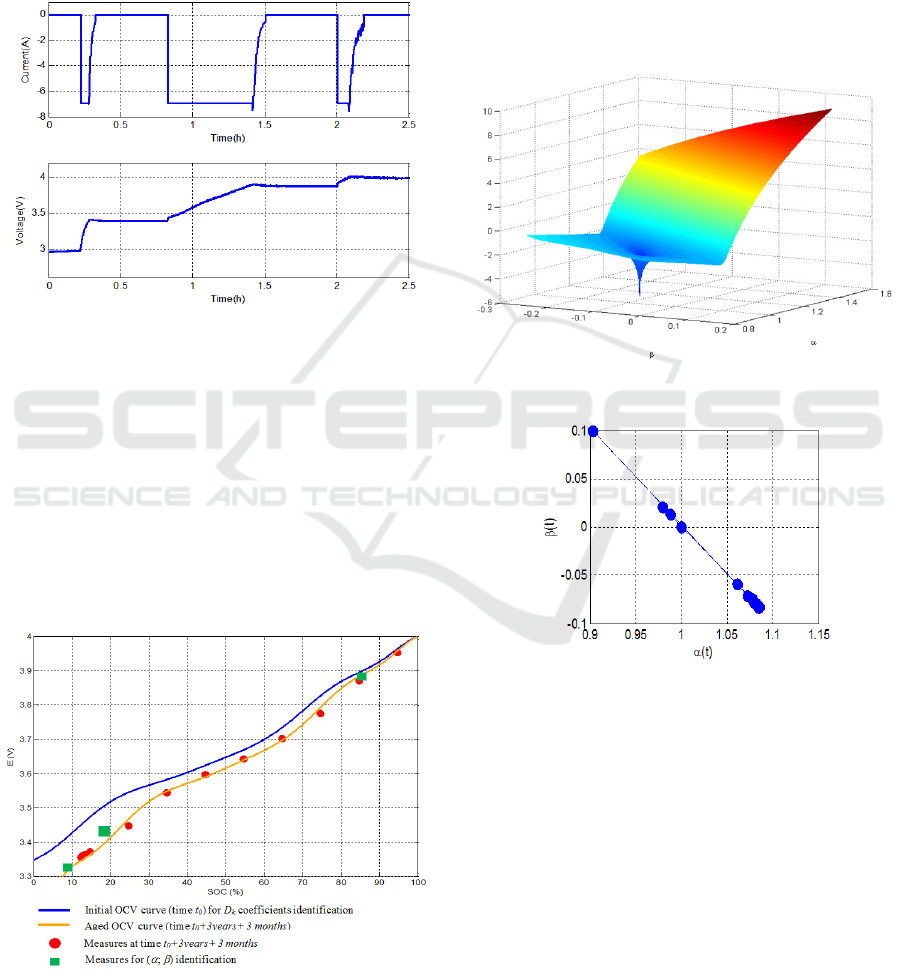
profile such as that shown in Figure 7. The pair (
,
) selected minimizes J
test
.
Figure 7: Charge profile example used to get the necessary
measures for the OCV curve adjustment.
To validate the pair (
,
) selected, the identified
OCV curve is compared with the measured OCV
curve in Figure 8. This figure shows the feasibility
of the parametrization given by relation (39) and
also shows that the proposed optimization leads to a
reliable reconstruction of the OCV curve over a wide
range of SOC and with a reduced number of voltage
measurements (namely three during on a charge
profile). Figure 9 shows the shape of the logarithm
of J
test
criterion that exhibits a global minimum.
Figure 8: Identification of the OCV curve using charge
profile measures and manual search of parameters
and
of a cell after two years calendar ageing.
The previous adjustment was performed for
several cell aging. From optimal identified pairs (
,
), figure 10 shows the variations of
as a function
of
. This figure shows that parameters
and
are
linked by the equation
= -
+ 1 which makes it
possible to write the relation:
11
SOCSOC
init
.
(41)
This remark permits to transform the OCV curve
adjustment problem after aging to the research for a
single parameter: parameter
.
Figure 9: Criterion J
test
as a function of the pair (
;
).
Figure 10: Variation of
as a function of
.
2.7 Unicity of Coefficient for Each
OCV Curve
Coefficient α characterizes the cell capacity loss and
is unique for each OCV curve. It is therefore an
aging indicator. The uniqueness of α is due to three
reasons:
1 - Polynomials defined by coefficients
init
k
D
(relation (27)) is strictly increasing.
2 -
11: SOCSOCT
is an application
strictly increasing and that defines a straight line
whose slope is α.
Lithium-ion Batteries Aging Motinoring Througth Open Circuit Voltage (OCV) Curve Modelling and Adjustment
63
3 - Equation
21
SOCESOCE
has an unique
solution
1
21
SOCSOC
.
Thus
= 1 corresponds to the initial ageing state;
> 1 indicates a cell capacity loss. The cell
may be considered to be aged.
3 OCV MODEL ADJUSTMENT AS
AGING
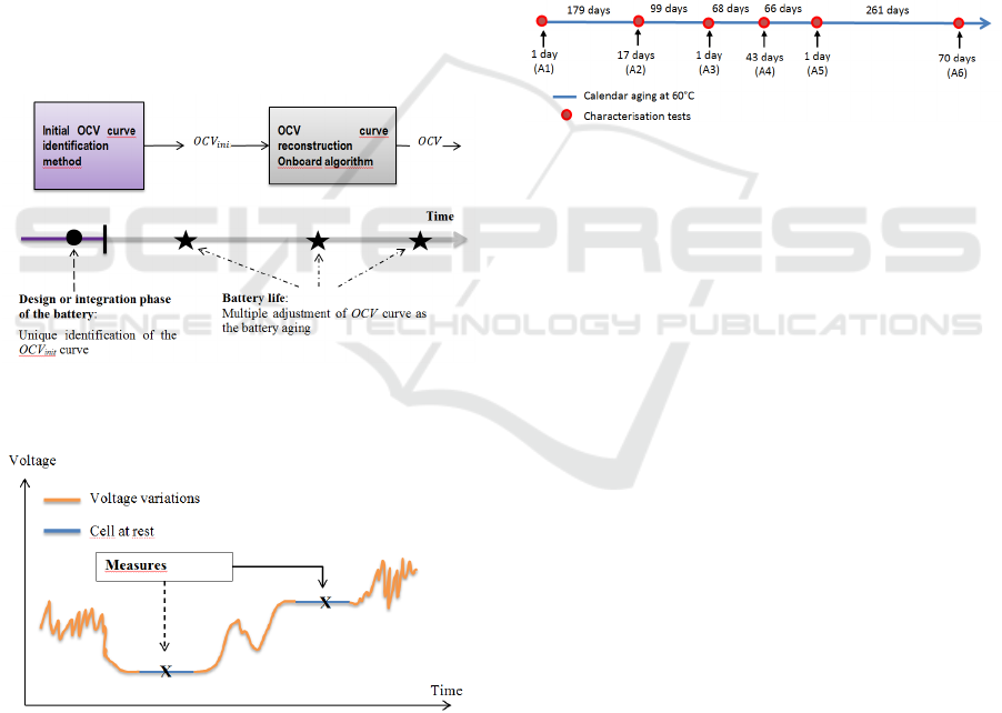
The proposed method has two steps illustrated in
figure 11. The first step is the identification of the
OCV curve at initial state (using relation (26) thus
leading to coefficients
init
k
D
). In the second step,
parameter characterizing the aging of the cell is
identified from at least two OCV measures in
normal operation or in specific operation (charge
phase for instance).
Figure 11: Block diagram of the OCV curve
reconstruction method during cell aging.
Figure 12: Description of measures and rest periods
required for the step two adjustments method
implementation.
To implement step 2 of figure 11 method, it is
require as shown in figure 12 to have two
consecutive rest periods that permits to measure the
cell OCV without the cell age has changed
significantly between the two measures.
3.1 Aging Characterization and Bench
Description
The strategy previously described is now applied to
a battery pack constituted of four 7 A.h VL6P type
lithium-ion cells from JCS-SAFT (LiNiCoAl
Oxide). The cells, numbered form 1 to 4, have
undergone an accelerated calendar aging at 60°C.
The aging phases are punctuated by characterization
tests. Characterization tests on Digatron bench
include measures of capacity, internal resistance and
OCV for each cell and for various temperatures. The
chronology of the aging and characterization tests is
given in Figure 13.
Figure 13: Chronology of calendar aging and
characterization tests.
3.2 Initial OCV Identification
Each battery cell initial OCV curve OCVC
init
must
be fitted by relation (27) before battery usage. This
necessary initial fitting can be time and resource
consuming but can be done off-line and is only once
realized.
However this relative complexity can be
reduced. Hypothesis 1 supposes that coefficients A
i,k
depend only on electrode electrochemistry and are
constant. Then, if the battery is made of the same
cells, the same initial OCV curve fitting should be
used for all the battery cells. If OCV curves are
different, these differences can be associated to
electrode stoichiometry dispersion in manufacturing.
These dispersions can be assimilated to aging
consequences and can be taken into account through
an appropriated parameter
.
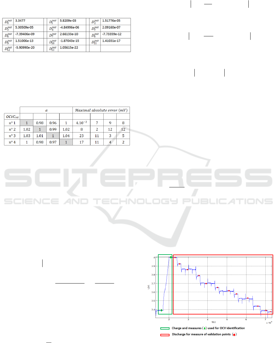
This result is verified with the 4 cells battery
pack. Table 1 shows that each OCVC
init
can be
obtained by the mapping of each other cell. This
table shows that a unique OCVC
init
can be used for
the 4 cells (with a maximal error less than the
measurement noise magnitude recorded when
implemented in a car). The cell2 OCVC
init
is defined
by (see relation (27)):
ICINCO 2016 - 13th International Conference on Informatics in Control, Automation and Robotics
64
N
k
kinit
kinit
SOCDE
0
(42)
with the following coefficients
will be used in the following.
Table 1: OCVC
init
fitting of 4 cells using a unique
polynomial and computation of parameter . The grey
boxes highlight the considered cell for polynomials fitting
for each experience. The fitting maximal absolute errors
are also gathered in the table for each experience.
3.3 OCV Curve Adjustment as Aging
The algorithm is based on the idea that for two OCV
voltages E
a
and E
b
such that E
a
< E
b
, the state of
charge variation
ba
EESOC ,
differs for each
aging state, especially if voltage E
a
and E
b
are very
different. This statement is demonstrated by
expressing the state of charge variation
ba
EESOC ,
at the initial state and for two other
aging states characterized by parameters
I
and
II
.
At initial state, state of charges leading to OCV E
a
and E
b
are denoted
init
a
SOC
and
init
b
SOC
and are
such that:
nom
EE
EE
nom
ba
init
a
init
b
init
ba
Q
I
Q
EEQ
SOCSOCEESOC
b
a
;
;
.
(43)
Let then SOC denotes the state of charge of an
aged cell and SOC
init
the state of charge of the same
unused battery for the same OCV. According to
relation (41), the two states of charge are linked by
the relation:
11
1
init
SOCSOC
.
(44)
At ageing state characterized by
I
, state of
charge variation between the two OCV E
a
and E
b
is
given by:
init
ba
I
ba
EESOCEESOC
I
;
1
;
.
(45)
Similarly, at ageing state characterized by
II
:
init
ba
II
ba
EESOCEESOC
II
;
1
;
.
(46)
Aging difference characterized by
III
implies a difference in state of charge variations:
III
SOCSOC
.
(47)
Thus, a measure
ba
EESOC ;;
corresponds to
an unique OCV curve. With a set of
2M
measures of state of charge variations
11
;
t
EESOC
with
M
EE ...
1
, there will be
1M
associated parameters
t
.
If the measures are perfects, all parameters
t
are
equals. If however measures are for instance marred
by noise, an optimal parameter α allowing to
accurately representing the experimental data must
be deduced. To solve this problem, a least square
problem can be formulated leading to the
minimization of the following criterion:
M
t
t
t
EESOC
EESOC
M
J
2
2
1
1
;;
;
1
1
.
(48)
3.4 Validation
The implementation of the OCV curve adjustment
algorithm previously described requires at least two
OCV measures. These measures are obtained here
on voltage profiles presented in Figure 14.
Figure 14: Example of charge profile providing two
measures for OCV curve reconstruction (second measure
at 4V) and OCV measure (during a discharge) for
validation.
Lithium-ion Batteries Aging Motinoring Througth Open Circuit Voltage (OCV) Curve Modelling and Adjustment
65

The charge part is used to get the two OCV
measures required for the curve adjustment. The
discharge part is used to get OCV measures required
to validate the method. During discharge, the
relaxation time after each step is about 30 minutes.
On the discharge part the SOC information required
for each validation points is calculated by current
integration from the reference point for SOC =
100% defined by E= E
100%
namely 4V.
Table 2 gives in column max(
) the 4 more
important errors (on all measures of the discharge)
and for 4 different temperatures. The column
Δ
gives voltages variations due to aging. These errors
are determined for the 6 aging denoted {A1, A2, A3,
A4, A5, A6} that appears in figure 13.
Table 2: Maximum identification errors for different
ageing and temperatures.
Figure 15: variation according to aging for different
temperatures.
Figure 15 shows parameter variations
according to temperature and cells aging. On this
figure,
parameter value grows according to
ageing. For cells 1, 3 and 4 the
values are more or
less equals. For cell2 case, the ageing is more
important and
is higher than 1.5 for measures at
A6.
Figure 15 shows that OCV curves are very little
affected by temperature, indeed no particular
variations are noted on the parameter
when
temperature is varying. The standard deviation, on
values, is higher for cell2 and on A4 measures (
A4
).
variations are mainly attributed to identification
errors.
4 CONCLUSIONS
The paper proposes a lithium-ion Open Circuit
Voltage (OCV) curve model that requires only one
parameter adjustment as batteries aging. Such a
result has been obtained through an analysis of
electrodes stoichiometries variations as ageing. A
two steps algorithm is then proposed for model
adjustment as aging. The first step is the
identification of the OCV curve at initial state. In the
second step, a parameter characterizing the aging of
the cell is identified from at least two OCV measures
in normal operation or in specific operation (charge
phase for instance). The efficiency of this algorithm
has been shown with a battery pack constituted of
four Lithium-ion cells. The modelling error remains
small in spite of cells aging and temperature
variations. Moreover, the OCV curve adjustment as
cell aging requires the optimization of only one
parameter and this parameter variations can be
correlated to battery aging. This parameter can thus
be viewed as a State Of Health (SOH) indicator.
The authors have recently proposed lithium-ion
cells models based on fractional differentiation
(Sabatier et al, 2014). They now intend to include
the OCV curve adjustment method proposed in this
paper into the cell model and also to propose
adjustment methods for the other model parameter in
order to get a cell model that is robust versus aging.
ACKNOWLEDGEMENTS
This work took place in the framework of the Open
Lab Electronics and Systems for Automotive
combining IMS laboratory and PSA Peugeot Citroën
company.
ICINCO 2016 - 13th International Conference on Informatics in Control, Automation and Robotics
66

REFERENCES
Armand M., Tarascon J. M., Building better batteries,
Nature 451, pp 652-657, 2008.
Arora, P, White R. E., Doyle M. Capacity Fade
Mechanisms and Side Reactions in Lithium-Ion
Batteries, Journal of the Electrochemical Society, Vol.
145, N° 10, pp. 3647–67.
Bard A. J., Inzelt G., Scholz F., Electrochemical
Dictionary Springer-Verlag Berlin Heidelberg. 2008.
Cheng M. W., Lee Y. S., Liu M., Sun C. C., State-of-
charge estimation with aging effect and correction for
lithium-ion battery, Electrical Systems in
Transportation, IET, Vol. 5, N° 2, 2015.
Dubarry M., Liaw B.Y., Identify capacity fading
mechanism in a commercial LiFePO4 cell, J. Power
Sources 194, pp 541-549, 2009.
Francisco J. M., Sabatier J., Lavigne L., Guillemard F.,
Moze M., Tari M., Merveillaut M., Noury A.,
Lithium-ion battery state of charge estimation using a
fractional battery model, IEEE International
Conference on Fractional Differentiation and its
Applications, 23-25 June 2014, Catania, Italy.
Honkuraa K., Honboa H., Koishikawab Y., Horibab T.,
State Analysis of Lithium-Ion Batteries Using
Discharge Curves, ECS Transaction, Vol. 13, pp 61-
73, 2008.
Hu Y., Yurkovich S., Guezennec Y., Yurkovich B.,
Electro-thermal battery model identification for
automotive applications, J. Power Sources 196, pp
449-457, 2011.
Karthikeyan D. K, Sikha G, White R. E., Thermodynamic
Model Development for Lithium Intercalation
Electrodes, J. Power Sources, 185: pp1398–1407.
2008.
Kim I. S., A Technique for Estimating the State of Health
of Lithium Batteries Through a Dual-Sliding-Mode
Observer, IEEE Transactions on power electronics,
Vol. 25, No. 4, April 2010.
Liaw B. Y., Dubarry M., in: G. Pistoia (Ed.), Electric and
Hybrid Vehicles: Power Sources, Models,
Sustainability, Infrastructure and the Market, Elsevier,
pp. 375-403, 2010.
Lee S., Kim J., Lee J., Cho B. H., State-of-charge and
capacity estimation of lithium-ion battery using a new
open-circuit voltage versus state-of-charge, Journal of
Power Sources, vol. 185, no. 2, pp. 1367–1373, 2008.
Petzl M., Danzer, M. A., Advancements in OCV
Measurement and Analysis for Lithium-Ion Batteries.
IEEE Transactions on Energy Conversion, 28(3),
pp.675–681., 2013.
Piller S., Perrin M., Jossen A., Methods for state-of-charge
determination and their applications, Journal of Power
Sources 96 (2001) 113-120, 2001.
Plett G. L., Extended Kalman filtering for battery
management systems of LiPB-based HEV battery
packs Part 3. State and parameter estimation, Journal
of Power Sources, 134, 277–292, 2004.
Pop V., Bergveldb H. J., Regtiena P. P. L., Op het Veldc J.
H. G., Danilovd D., Notten P. H. L., Battery Aging
and Its Influence on the Electromotive Force. Journal
of The Electrochemical Society, 154(8), p.A744-A750,
2007.
Roscher M.A., Assfalg J., Bohlen O.S., Detection of
Utilizable Capacity Deterioration in Battery Systems,
IEEE Trans. Veh. Technol. 60 pp. 98-103, 2011.
Roscher, M.A., Bohlen, O., Vetter, J., OCV Hysteresis in
Li-Ion Batteries including Two-Phase Transition
Materials, International Journal of Electrochemistry,
pp.1–6,2011.
Sabatier J., Merveillaut M., Francisco J., Guillemard F.,
Lithium-ion batteries modelling involving fractional
differentiation, Journal of power sources, 262C, pp.
36-43, 2014.
Sabatier J., Francisco J., Guillemard F., Lavigne L., Moze
M., Merveillaut M., Lithium-ion batteries modelling: a
simple fractional differentiation based model and its
associated parameters estimation method, Signal
Processing, Vol 207, pp. 290-301, 2015.
Santhanagopalan S., White R. E., Online estimation of the
state of charge of a lithium ion cell, Journal of Power
Sources 161, pp 1346-1355, 2006.
Schmidt, J.P., Tran H. Y., Richtera J., Ivers-Tifféea E.,
Wohlfahrt-Mehrensb M., Analysis and prediction of
the open circuit potential of lithium-ion cells. Journal
of Power Sources, 239, pp.696–704, 2013.
Weng C, Sun J., Peng H., A unified open-circuit-voltage
model of lithium-ion batteries for state-of-charge
estimation and state-of-health monitoring, Journal of
Power Sources, vol. 258, pp. 228-237, 2014.
Lithium-ion Batteries Aging Motinoring Througth Open Circuit Voltage (OCV) Curve Modelling and Adjustment
67
