
MYNTS: Multi-phYsics NeTwork Simulator
Tanja Clees, Kl
¨
are Cassirer, Nils Hornung, Bernhard Klaassen, Igor Nikitin, Lialia Nikitina,
Robin Suter and Inna Torgovitskaia
Fraunhofer Institute for Algorithms and Scientific Computing, Schloss Birlinghoven, 53754, Sankt Augustin, Germany
Keywords:
Simulation Tools and Platforms, Complex Systems Modeling and Simulation, Optimization of Non-Linear
Systems, Simulation of Transport Networks.
Abstract:
We present a generic approach for the simulation of transport networks, where the steps of physical modeling
and numerical simulation are effectively separated. The model is described by a list of physical equations and
inequalities as problem constraints for non-linear programming (NLP). This list is translated to the language of
expression trees and is made accessible for the numerical solution by standard NLP solvers. Various problem
types can be solved in this way, including stationary and transient network simulation, feasibility analysis and
energy-saving optimization. The simulation is provided for different disciplines, such as gas transport, water
supply and electric power networks. We demonstrate the implementation of this approach in our multiphysics
network simulator.
1 INTRODUCTION
The simulation of transport networks in civil engi-
neering becomes increasingly important for the plan-
ning and stable operation of modern infrastructure.
Many software systems exist for the solution of spe-
cialized problems in the simulation of gas transport
networks (Scheibe and Weimann, 1999; Aymanns
et al., 2008), water supply (Rogalla and Wolters,
1994; Stevanovic et al., 2009), electric power trans-
mission (Milano, 2015; Zimmerman and Murillo-
Sanchez, 2015), etc. Our purpose is to develop a uni-
versal system capable of solving all problems of this
kind, as well as of providing for them an energetically
efficient optimal solution. The system has to be max-
imally open in terms of mathematical modeling and
numerical solver, allowing the user to extend the sys-
tem by new element types and new conditions and to
upgrade it by modern highly efficient algorithms.
The possibility of such a universal solution fol-
lows from the great similarity of the considered prob-
lems. Indeed, different network disciplines represent
the network topology as a graph on which problems
of the following types are formulated:
• stationary problems – systems of non-linear equa-
tions f (x) = 0;
• transient problems – differential-algebraic equa-
tions, DAEs, f (x, ˙x) = 0;
• feasibility problems – find (any) solution of the
system of equations and inequalities f (x) = 0,
g(x) ≥ 0;
• constrained optimization – find min h(x) such that
f (x) = 0, g(x) ≥ 0.
Note that constrained optimization is the most general
formulation, while the three others represent its par-
ticular cases: stationary problems – in the absence of
the inequalities g(x) ≥ 0 and with a trivial objective
function h(x) one has to solve only non-linear sys-
tems f (x) = 0; the sequential solution of non-linear
systems represents a process of (semi-)implicit inte-
gration of a DAE; feasibility problems also belong to
constrained optimization, where one can select an ar-
bitrary objective function.
In its most general form constrained optimization
is also known as non-linear programming, NLP, for
which, since the 1970s, many efficient algorithms
have been developed (Bazaraa and Shetty, 1979; Bert-
sekas, 1999; Avriel, 2003; Fletcher, 2013) and imple-
mented in a number of software packages (Murtagh
and Saunders, 1978; Gill et al., 2005; W
¨
achter and
Biegler, 2006; Nocedal and Wright, 2006; Belotti
et al., 2013). Nowadays the solution of the above
listed problems is as easy as the solution of a linear
sparse system, one only needs to represent the prob-
lem in a standard form, accepted by the correspond-
ing software package. Continuing this analogy, the
solution of a linear sparse system requires to spec-
ify the system matrix in a triplet, a column or a row
Clees, T., Cassirer, K., Hornung, N., Klaassen, B., Nikitin, I., Nikitina, L., Suter, R. and Torgovitskaia, I.
MYNTS: Multi-phYsics NeTwork Simulator.
DOI: 10.5220/0005961001790186
In Proceedings of the 6th International Conference on Simulation and Modeling Methodologies, Technologies and Applications (SIMULTECH 2016), pages 179-186
ISBN: 978-989-758-199-1
Copyright
c
2016 by SCITEPRESS – Science and Technology Publications, Lda. All rights reserved
179
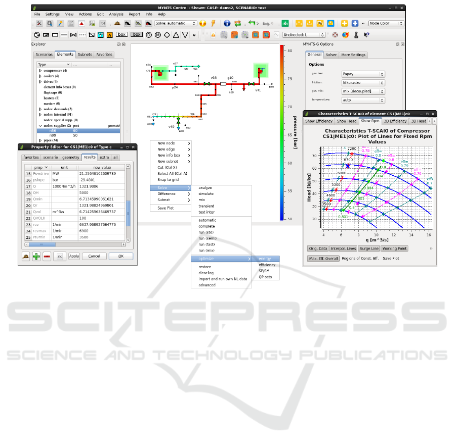
Figure 1: Gas transport network simulation in Mynts.
compressed form, while NLP solvers accept systems
of non-linear equations in the form of so-called ex-
pression trees (Gay, 2005). This de facto standard
is supported by many existing NLP solvers, while
newly developed algorithms can be easily equipped
with the necessary interface. In this way the mathe-
matical modeling becomes effectively separated from
the solution algorithms, providing the required flexi-
bility and modularity of the software.
The same transport network problem can have var-
ious representations: a human-readable description of
the network (e.g. in NetList format, used in prac-
tice for solution of real-life problems for gas, water
and electric power transport (Baumanns et al., 2012;
Clees, 2012; Clees, 2016; Clees et al., 2016a; Clees
et al., 2016b)), formats understandable only by sim-
ulation kernels (e.g. NL (Gay, 2005)), there is also
an intermediate level of modeling languages (such
as AMPL (Fourer et al., 2002), Modelica (Modelica,
2012)). Well designed simulator should be able to
translate the problem between its different represen-
tations and do it fast for large realistic problems. In
this paper we describe the algorithms suitable for this
purpose.
Related work: in (Clees, 2012) we present gen-
eral concepts common for all types of transport net-
work problems, in (Clees, 2016) we describe the gas
part of our simulator applied for parameter studies in
gas transport networks, in (Clees et al., 2016a; Clees
et al., 2016b) the detailed modeling of water cool-
ing networks is given. Our advancement reported in
the present paper is the development of general algo-
rithms for formulation and solution of transport net-
work problems based on their representation in NLP
form. In the first place, we have the task to translate
between different problem encodings, i.e., between a
human-readable description of the transport network
problem and the language understood by NLP solvers.
We tackle these aspects in Section 2. Different ap-
proaches for solving NLPs are discussed in Section 3.
Our system Mynts with its main components and ex-
amples of usage is presented in Section 4.
2 PROBLEM FORMULATION
Network problems can be presented as a list of ele-
ments (nodes, edges), containing a topological defi-
nition (in the form of an incidence matrix, i.e., every
edge should refer to the two nodes it connects to) and
a set of properties used for problem formulation (e.g.,
node coordinates, pipe length, diameter, etc). For in-
stance, a gas transport problem can have the following
form.
SIMULTECH 2016 - 6th International Conference on Simulation and Modeling Methodologies, Technologies and Applications
180

Network base description:
# Nodes
n, name="n56", H=5.2, X=14400, Y=10800
n, name="n99", H=0, X=18471.821, Y=10670.833
....
# Pipes
p, name="p11", node1="n93", node2="n94",
L=7900.0, D=0.5, k=0.02
p, name="p12", node1="n94", node2="n52",
L=4700.0, D=0.5, k=0.02
....
# Compressors
c, name="CS1|ME1|c0", node1="CS1|ME1|n2",
node2="CS1|ME1|n3"
c, name="CS1|ME2|c0", node1="CS1|ME2|n4",
node2="CS1|ME2|n5"
....
For user convenience, this description can be divided
into sections where the properties for a class of prob-
lems are listed (base) and where problem variations
are set (scenario). They can also be stored in separate
files.
Network scenario description:
name="n56", PSET=50, gasmix="gas1"
name="n99", PSET=60, gasmix="gas2"
name="n76", QSET=300
name="n91", QSET=1000
name="CS1|ME1|c0", MODE="PO", SPO=80,
model="advanced", cchar="T-SCAI0",
echar="P-SCAI0"
name="CS1|ME2|c0", MODE="M", SM=500,
model="advanced", cchar="T-SCAI1",
echar="P-SCAI1"
A scenario for a gas transport problem typically con-
tains pressure settings in supply nodes (PSET), out-
flow settings in exit nodes (QSET), references to
gas composition (gasmix), compressor mode settings,
such as output pressure (SPO) and output flow (SM),
a model of operation (advanced or free), a reference
to characteristics of compressor (cchar) and its driv-
ing engine (echar), etc. Any properties can be added,
they should only make sense in the context of the con-
sidered discipline.
The discipline description is a list of translation
rules, which allow to compose variables, equations
and inequalities given per element.
Network discipline description:
# Variables
for every node:
var P,rho,T,...
# pressure, density, temperature
for every edge:
var Q... # flow
for every compressor:
var Rev,Perf,Had...
# revolutions per minute, power,
# adiabatic enthalpy difference
.....
# Equations
for every node:
eq gas_law(rho,P,T, gasmix,...)=0
for every pipe:
eq pipe_law(P@node1,P@node2,Q, L,D,...)=0
.....
Here the section of variables extends the list of prop-
erties per given element by new properties whose
values will be computed in the network simulation.
Equation prototypes combine the properties with ex-
pressions representing the underlying physical laws.
Gas transport simulation can use several types of laws
for gas compressibility, pressure drop in pipes and
compressor working conditions, in more detail con-
sidered in Section 4. They can also be extended by
the user, by specifying a formula per element or a
class of elements. Let us demonstrate this by defin-
ing a quadratic pipe law (Mischner et al., 2011) by
the equation:
pow(P@node1,2)-pow(P@node2,2)-R*Q*abs(Q)=0
A translation utility represents this equation in the
form of an expression tree:
then, using the correspondence
P@node1 P@node2 Q R 2
v1 v2 v3 n0.1 n2
pow abs * -
o5 o15 o2 o1
the tree is traversed by the left-hand rule and encoded
in Polish prefix notation (PPN):
o1 o1 o5 v1 n2 o5 v2 n2 o2 o2 v3 o15 v3 n0.1
In the obtained representation of the expression tree
the leaves are variables (v...) and constants (n...),
while the branches are operators (o...). A represen-
tation in the form of an expression tree makes equa-
tions suitable for automatic differentiation using the
chain rule. A detailed description of the encoding
procedure can be found in (Gay, 2005). The interface
MYNTS: Multi-phYsics NeTwork Simulator
181

supports more than 70 basis operators and a possibil-
ity to extend them by arbitrary user defined functions.
PPN encoded expression trees are the language which
many NLP solvers understand.
In terms of general theory (Harrison, 1978) all
these representations belong to formal languages, be-
ing sets of strings of symbols, constrained by specific
rules. The network description and the lists of equa-
tions in human-readable or NLP format define differ-
ent formal languages, while the description of the dis-
cipline provides a means for translation, in a way:
discipline ∗ network description = NLP.
Algorithmically, this can be done as follows.
Algorithm 1: Problem translation.
read network graph (base and scenario);
read vars and eqs prototypes (discipline);
translate eqs prototypes to NLP format
with placeholders for vars and consts;
loop over element:
create vars per element according
to the discipline description;
place them into the graph as sequentially
numbered ids (v1...vn);
loop over element:
create eqs per element according to
the discipline description;
substitute actual vars and consts
to the placeholders;
output the eqs.
Since the main part of the algorithm is a straightfor-
ward substitution (stamping), it requires O(N + E)
operations, where N and E are the numbers of nodes
and edges in the network graph, respectively.
3 PROBLEM SOLUTION
In the field of applied optimization the problems are
often subdivided into two parts: simulation and opti-
mization. Simulation solves the part of the problem
defined by equations f (x, y) = 0 with respect to some
part of the variables y, while the remaining variables
x are considered as constant parameters. Then opti-
mization is applied to the objective function h(x, y),
with respect to the variables x, while y is permanently
updated for the given x using the simulation. Algo-
rithmically this can be expressed as follows.
Algorithm 2: Optimization on top of the simulation.
define y(x):
solve f(x,y) w.r.t. y;
return y;
optimize h(x,y(x)) w.r.t. x.
An alternative is to use NLP algorithms which solve
the optimization and simulation parts simultaneously.
Algorithm 3: NLP.
optimize h(x,y) w.r.t. (x,y) s.t. f(x,y)=0.
The first variant is often used if the simulation and/or
the optimization are considered as blackbox algo-
rithms, e.g., if simulation y(x) is encapsulated in a
proprietary software tool. In this case one is re-
duced to applying the first algorithm indeed. The
second variant composes a unified system of equa-
tions f (x, y) = 0 and optimality conditions for h(x, y),
which are solved simultaneously by means of super-
convergent methods (usually a stabilized Newton’s
method). The first algorithm finds, for every value
of x, an exact solution of the system f (x, y) = 0. This
is completely superfluous for intermediate optimiza-
tion steps when x is only an approximation to the
optimum. For the second algorithm the precision of
the solution for the equations and the precision of the
optimality conditions are improved simultaneously in
the solution process, so that a precise solution of the
simulation problem is obtained only at the last step,
being also the optimal one. For the first algorithm
the required computational effort can be estimated as
O(Nsim Nopt), where Nsim is the number of itera-
tions per simulation and Nopt is the number of op-
timization steps. The second algorithm solves a uni-
fied system, which is almost entirely composed of the
equations from the simulation part, so that the over-
head related to the optimality conditions is usually
small and the overall effort becomes O(Nsim). Thus,
NLP algorithms definitely win in performance and,
therefore, they are our preferred choice.
The possibility to represent gas network simu-
lations in NLP form has been earlier discussed in
(Schmidt et al., 2015a), where the mathematical mod-
eling of gas transport networks has been considered in
great detail. However, the implementation (Schmidt
et al., 2015b) used the simplest possible NLP ver-
sion, a penalty method, taking a cumulative norm of
the residuals of the physical equations as single ob-
jective function. This approach admits a violation of
the physical constraints (gas laws, etc). Although the
global minimum of this objective coincides with the
solution for feasible problems, there is danger that the
solution process gets stuck in a local minimum and
the physical solution will be lost. Also, one cannot
simply add a real objective there, like the total power
of all compressors in energy optimization, since the
improvement of the objective would be achieved at
the cost of the violation of the physical equations.
Fortunately, this is easy to correct and in our imple-
mentation all physical equations are set as equality
SIMULTECH 2016 - 6th International Conference on Simulation and Modeling Methodologies, Technologies and Applications
182

constraints f (x) = 0 and, at solutions, are satisfied ex-
actly.
For solving NLPs many efficient algorithms have
been developed (Bazaraa and Shetty, 1979; Bertsekas,
1999; Avriel, 2003; Fletcher, 2013), e.g., those imple-
mented in the optimization package Ipopt (W
¨
achter
and Biegler, 2006):
• an interior-point algorithm (also known as primal-
dual barrier method) for the solution of generic
NLPs with equations and inequalities;
• a line-search filter with second order corrections,
serving as a stabilizer for Newton’s method;
• an inertia correction method, driving the iterations
towards a critical point of the desired type (e.g.,
minimum, not maximum, not saddle point);
• a feasibility restoration method, applying an
emergency restart in the case that the convergence
becomes too slow;
• an automatic initialization, appropriate problem
scaling, interfaces to many sparse linear solvers,
etc.
Our approach, using the translation of network
problems to the standard NLP format, also allows to
employ for their solution any other package, such as
Snopt (Gill et al., 2005), Minos (Murtagh and Saun-
ders, 1978), Knitro (Nocedal and Wright, 2006), etc.
For the solution of mixed integer NLPs one can use
Couenne (Belotti et al., 2013), while multiobjective
optimization can be done with the approaches de-
scribed in (Clees et al., 2015).
4 NETWORK SIMULATION IN
MYNTS
The backbone of the system is formed by linear
Kirchhoff equations and non-linear element equa-
tions, depending on the flow through an element and
on its two adjacent nodal variables:
∑
e
I
ne
Q
e
= Q
(s)
n
, f
e
(P
in
, P
out
, Q
e
) = 0, (1)
where indices n = 1...N denote the nodes and e =
1...E the edges of the network graph, I
ne
is the in-
cidence matrix of the graph, Q
e
are flows through the
edges, Q
(s)
n
are source/sink contributions, localized in
the supply/exit nodes, P
n
are nodal variables (pres-
sure, voltage, etc – depending on the discipline). For
example, in gas transport networks the simplest pipe
law has a quadratic form (Mischner et al., 2011):
f
e
= P
2
in
− P
2
out
− RQ
e
|Q
e
|, (2)
where R is a resistance coefficient, depending on pipe
length L, diameter D, friction factor λ, temperature
T , compression factor z and on pressure, temperature
and density at normal conditions (P
norm
, T
norm
, ρ
norm
):
R =
16 λ L T z P
norm
ρ
norm
π
2
D
5
T
norm
. (3)
System (1) describes a stationary network problem,
while for dynamical (transient) problems additional
terms with time derivatives are included. Specific for
every medium, new equations can be introduced, re-
lating additional nodal and element variables.
Modeling of gas transport networks in Mynts includes
the following building blocks, described in detail in
(Schmidt et al., 2015a; Mischner et al., 2011; CES,
2010):
• main elements: supplies, exits, pipes, valves,
compressors, drives, regulators, resistors, short-
cuts, flaptraps, heaters, coolers;
• gas laws: ideal, AGA, Papay, AGA8-DC92 (ISO
standard);
• pressure drop in pipes: besides the quadratic law,
more accurate Hofer and Nikuradze formulae are
used;
• various models for compressors (turbo, piston)
and their drives (gas turbine, steam turbine, gas
motor, electro motor), with characteristic dia-
grams calibrated on real compressors;
• control logic of compressors and regulators, im-
plemented in the form of control equations or in-
equalities, e.g., a compressor/regulator can have a
control goal to keep fixed output pressure (SPO),
input pressure (SPI) or flow value (SM);
• gas temperature: propagation over the network,
including non-linear heat capacity, heat exchange
with the soil, Joule-Thomson effect (temperature
drop in gas due to free expansion through a valve,
regulator, etc);
• gas composition: propagation and mixing (includ-
ing detailed molar components and effective gas
properties like critical temperature and pressure,
calorific value, molar mass, etc).
Modeling of water networks strongly resembles the
modeling of gas transport networks, except that a set
of important simplifications can be applied. In Mynts
it is assumed, e.g., that transient effects and the com-
pressibility of the fluid do not play a role. Hence,
the constitutive assumption, which relates the pres-
sure to the density of a compressible fluid, is omitted.
Moreover, only the temperature is considered as inter-
nal energy and only one phase of liquid water is be-
ing modeled. Mynts includes the following building
MYNTS: Multi-phYsics NeTwork Simulator
183
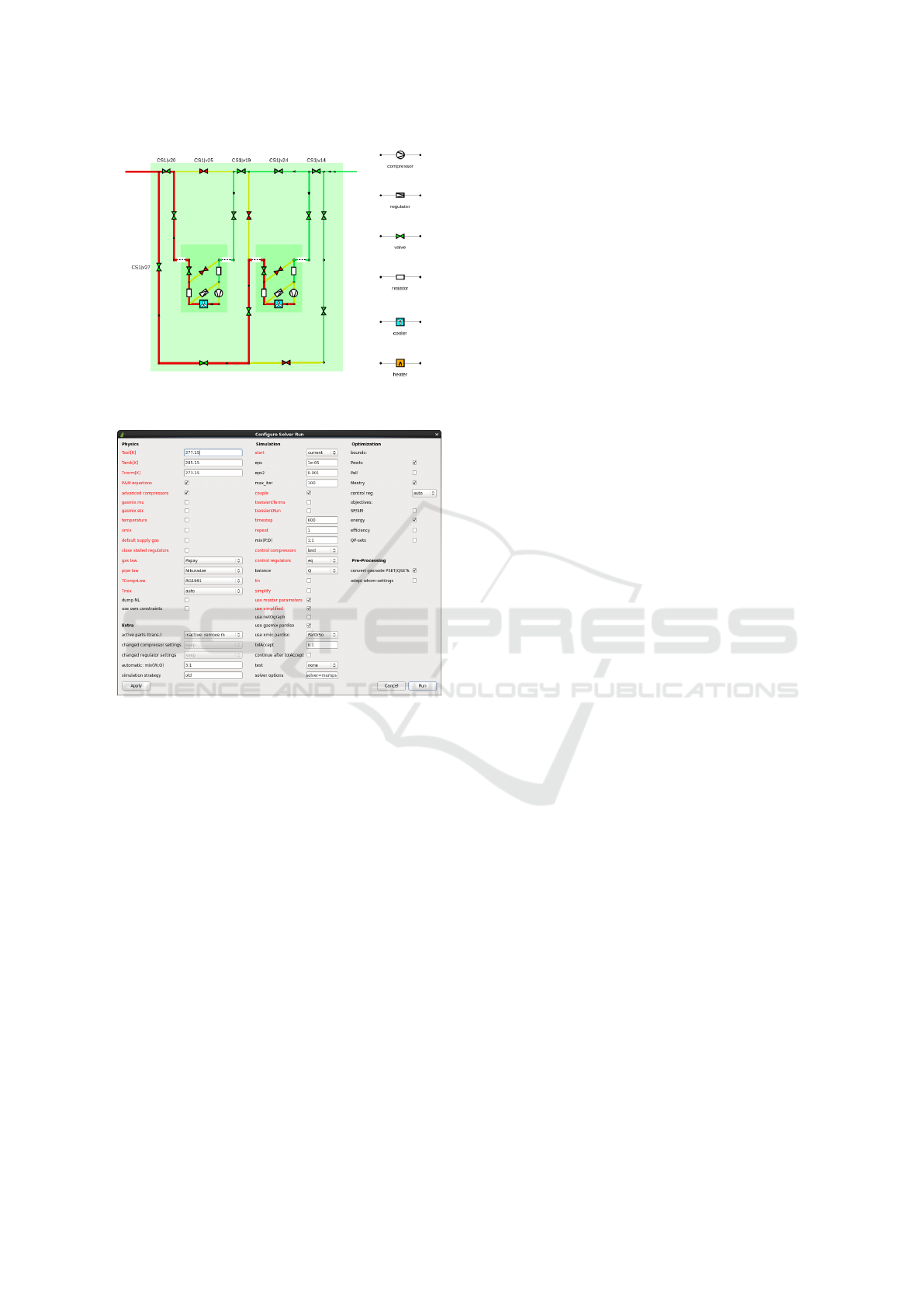
Figure 2: Gas transport network simulation in Mynts.
Closeup to a compressor station.
Figure 3: Gas transport network simulation in Mynts. Con-
figuration of the solver.
blocks, which are described in detail in (Clees et al.,
2016a; Clees et al., 2016b; Colburn, 1933; Colebrook,
1939; VDI/VDE, 1962; KSB AG, 2005; Brki
´
c, 2011):
• main elements: supplies, exits, pipes, resistors,
two-way and three-way valves, pumps and heat
exchangers;
• pressure drop in pipes: Bernoulli’s equation with
friction including a variety of implementations for
Colebrook’s friction factor (more complex arma-
tures are considered as simple resistors via their
k
vs
-values);
• models for regulated and unregulated pumps (in-
cluding user defined characteristic curves), heat
exchangers and two-way or three-way valves with
linear and equal percentage characteristics;
• simple control via goals defined either for pump
speed or valve lift, or – at arbitrary elements of the
network – for pressure, pressure drop, flow rate or
temperature;
• water temperature: propagation and mixing over
the network, power supply and exit at dedicated
elements, heat exchange with the environment
and with other network elements.
Modeling of electric power networks (Herman, 2011;
Milano, 2010):
• main elements: buses (generators, consumers,
prosumers, internal) and branches (transmission
lines, transformers and phase shifters, shortcuts);
• voltage drop in lines due to resistances (direct-
current, DC) or impedances (alternating-current,
AC): analogously to Ohm’s law for DC circuits,
the voltage drop in an AC circuit is the product
of the current and the impedance of the circuit;
electrical impedance is the vector sum of electri-
cal resistance, capacitive reactance and inductive
reactance;
• Norton scheme (admittance formulation): all con-
stant impedance elements of the model are in-
corporated into a complex bus admittance matrix
that relates the complex nodal current injections to
the complex node voltages; similarly, the system
branch admittance matrices relate the bus voltages
to the vectors of branch currents at the from and
to ends of all branches, respectively;
• various types of transformers, their parameters
(e.g. tap ratio, phase shift) and connections
(Delta, Wye, Wye-G).
Fig. 1 shows an example of a gas transport simula-
tion in Mynts. The network, used here for illustration,
contains 100 nodes, 111 pipes and other connecting
elements. We note that real life problems are much
larger. In cooperation with our partners we solve sta-
tionary and transient problems for gas networks with
thousands of elements.
The color in Fig. 1 shows the pressure distribution
in the network, which starts from 50bar and 60bar,
respectively, at the two supply nodes, is increased to
80bar by two compressor stations and then gradually
falls to 55bar at the exit nodes.
On the bottom right a characteristic diagram of
one compressor is shown, where the horizontal axis
refers to the volume flow through the compressor, the
vertical axis to the adiabatic enthalpy difference, the
blue parabolic curves correspond to fixed revolution
numbers, the magenta and dark cyan lines to fixed adi-
abatic efficiency, the green line to maximal efficiency
and the red line to the minimal possible throughput
flow for the given pressure increase (the so-called
surge line). The curves for the maximal and the min-
imal revolution numbers and the surge line define a
working region of the compressor, where the working
SIMULTECH 2016 - 6th International Conference on Simulation and Modeling Methodologies, Technologies and Applications
184

point must be located (shown by a blue cross, here lo-
cated on the surge line). In addition, there is an upper
limit for the power, provided by the compressor drive,
and there are lower and upper limits on input and out-
put pressure and flow, which together with other con-
trol equations and inequalities contribute to the whole
NLP system.
The solution of the NLP system can either be per-
formed as a “pure simulation” (solve>simulate) or as
a simulation with optimization (solve>optimize). For
the optimization the following objectives can be se-
lected:
• energy: minimize the total power, provided by all
drives;
• efficiency: maximize the average adiabatic effi-
ciency for all compressors;
• SPSM: minimize the deviation from the pre-
scribed pressure and flow conditions in compres-
sors and regulators (SPO, SPI, SM);
• QP-sets: minimize the deviation from the pre-
scribed flow settings (QSET) for supply nodes
with the given pressure settings (PSET).
The energy optimization allows to achieve the best en-
ergy savings of the gas transport for a given network
scenario. The efficiency optimization tries to set all
compressors on their central green lines. The opti-
mization of SPSM/QP-sets allows to control the dis-
tribution of load between compressors/suppliers.
Fig. 2 shows a closeup of a compressor station.
It consists of two compressors, which by means of
a special pattern of open and closed valves are con-
nected parallel to each other. Each compressor has in-
put and output resistors and is equipped with a cooler,
compensating the temperature increase in the com-
pressor, and a bypass regulator. This regulator is au-
tomatically opened if the working point reaches the
surge line and provides an internal gas circulation to
keep a constant output pressure for small outflows.
There is also a bypass valve, which opens only if the
compressor is shut down.
Fig. 3 shows a menu for detailed solver configu-
ration. In particular, it allows to set various physi-
cal parameters, switch between the physical models,
add transient terms, choose a solution method (e.g.,
the whole problem can be solved as a coupled sys-
tem at once or in blocks using an iterative relaxation
scheme), set the maximal number of iterations, the
solver tolerance, select deep options to the solver, etc.
The optimization part allows to select the above de-
scribed objectives or their combinations.
The viewer visualizes the network hierarchically,
switching automatically the level of detail suitable for
the current zoom factor. The user can select a property
shown on the graph by color or by the variable width
of the edges and nodes, change the size and shape of
visual elements, the detailization of the displayed in-
formation, etc.
Graphical user interface of Mynts is not only a net-
work viewer, but also a scalable network editor. It al-
lows to create and modify the network topology (new
nodes/edges, connect, merge, split, etc) and also to
edit the properties of the elements. For example, the
left bottom menu in Fig. 1 shows the details of a com-
pressor element, where the user can inspect different
properties and modify the settings.
The detailed numbers on Mynts performance are
given in our satellite paper (Clees et al., 2016c). In
particular, solution of a realistic gas transport network
scenario with 4466 nodes and 5362 edges requires
1.9sec on a 3 GHz Intel i7 CPU.
5 CONCLUSIONS
We have presented a generic approach for the simula-
tion of transport networks. The main steps of physi-
cal modeling and numerical simulation are effectively
separated. Input data for the modeling come in the
form of lists representing the topology of the network,
physical properties of the elements and a prototypical
description of variables and constraints defining the
discipline. A rapid algorithm translates the problem
statement into the language of PPN encoded expres-
sion trees, making it accessible for the numerical so-
lution by standard NLP solvers. The applicability of
this approach has been demonstrated on various prob-
lem types, including stationary and transient network
simulation, feasibility analysis and energy-saving op-
timization. The approach has been implemented in
our multiphysics network simulator Mynts, support-
ing various disciplines, such as gas transport, water
supply and electric power networks.
Our further plans include the support of other dis-
ciplines (steam engines, mechanical transmissions,
pipelines in the chemical industry), the solution of
cross-disciplinary problems and interfacing to other
simulation kernels and modeling systems (Couenne,
SCIP, Modelica).
REFERENCES
Avriel, M. (2003). Nonlinear Programming: Analysis and
Methods. Dover Publishing.
Aymanns, P. et al. (2008). Online simulation of gas dis-
tribution networks. 9th SIMONE Congress, October
15–17, 2008, Dubrownik, Croatia.
MYNTS: Multi-phYsics NeTwork Simulator
185

Baumanns, S. et al. (2012). MYNTS User’s Manual, Release
1.3. Fraunhofer SCAI.
Bazaraa, M. S. and Shetty, C. M. (1979). Nonlinear pro-
gramming: theory and algorithms. John Wiley &
Sons.
Belotti, P. et al. (2013). Mixed-integer nonlinear optimiza-
tion. Acta Numerica, 22:1–131.
Bertsekas, D. P. (1999). Nonlinear Programming. Athena
Scientific.
Brki
´
c, D. (2011). Review of explicit approximations to
the Colebrook relation for flow friction. Journal of
Petroleum Science and Engineering, 77(1):34–48.
CES (2010). DIN EN ISO 12213-2: Natural gas – Calcula-
tion of compression factor. European Committee for
Standardization.
Clees, T. (2012). MYNTS – Ein neuer multi physikalis-
cher Simulator f
¨
ur Gas, Wasser und elektrische Netze.
Energie-Wasser Praxis, (09):174–175.
Clees, T. (2016). Parameter studies for energy networks
with examples from gas transport. Springer Proceed-
ings in Mathematics & Statistics, 153:29–54.
Clees, T. et al. (2015). RBF-metamodel driven multiobjec-
tive optimization and its application in focused ultra-
sonic therapy planning. In R
¨
uckemann, C.-P., editor,
ADVCOMP 2015, The Ninth International Confer-
ence on Advanced Engineering Computing and Appli-
cations in Sciences, July 19–24, 2015, Nice, France,
pages 71–76. International Academy, Research, and
Industry Association.
Clees, T. et al. (2016a). Cooling circuit simulation I: Mod-
eling. Technical Report, Fraunhofer SCAI.
Clees, T. et al. (2016b). Cooling circuit simulation II: A nu-
merical example. Technical Report, Fraunhofer SCAI.
Clees, T. et al. (2016c). A globally convergent method for
generalized resistive systems and its application to sta-
tionary problems in gas transport networks. In Proc.
SIMULTECH 2016, July 29–31, 2016, Lisbon, Portu-
gal (accepted).
Colburn, A. P. (1933). Mean temperature difference and
heat transfer coefficient in liquid heat exchangers. In-
dustrial & Engineering Chemistry, 25(8):873–877.
Colebrook, C. F. (1939). Turbulent flow in pipes, with par-
ticular reference to the transition region between the
smooth and rough pipe laws. Journal of the Institu-
tion of Civil Engineers, 11(4):133–156.
Fletcher, R. (2013). Practical Methods of Optimization.
John Wiley & Sons.
Fourer, R. et al. (2002). AMPL: A Modeling Language for
Mathematical Programming. Cengage Learning, 2nd
edition.
Gay, D. M. (2005). Writing .nl Files. Technical Report,
Sandia National Laboratories, Albuquerque.
Gill, P. E. et al. (2005). SNOPT: An SQP algorithm for
large-scale constrained optimization. SIAM Review,
47(1):99–131.
Harrison, M. A. (1978). Introduction to Formal Language
Theory. Addison-Wesley.
Herman, S. L. (2011). Delmar’s Standard Textbook of Elec-
tricity. Delmar.
KSB AG (2005). Auslegung von Kreiselpumpen. KSB Ak-
tiengesellschaft, 5th edition.
Milano, F. (2010). Power System Modelling and Scripting.
Springer, Berlin, Heidelberg.
Milano, F. (2015). PSAT Software. faraday1.ucd.ie/psat
.html.
Mischner, J. et al. (2011). Systemplanerische Grundla-
gen der Gasversorgung. Oldenbourg Industrieverlag
GmbH.
Modelica (2012). A Unified Object-Oriented Language for
Systems Modeling. Modelica Association.
Murtagh, B. and Saunders, M. (1978). Large-scale lin-
early constrained optimization. Mathematical Pro-
gramming, 14:41–72.
Nocedal, J. and Wright, S. J. (2006). Numerical Optimiza-
tion. Springer.
Rogalla, B.-U. and Wolters, A. (1994). Slow transients
in closed conduit flow – part I: Numerical meth-
ods. In Chaudhry, M. H. and Mays, L. W., editors,
Computer Modeling of Free-Surface and Pressurized
Flows, volume 274 of NATO ASI Series, pages 613–
642. Springer, Netherlands.
Scheibe, D. and Weimann, A. (1999). Dynamische Gas-
netzsimulation mit GANESI. GWF Gas/Erdgas,
(9):610–616.
Schmidt, M. et al. (2015a). High detail stationary optimiza-
tion models for gas networks: model components. Op-
timization and Engineering, 16(1):131–164.
Schmidt, M. et al. (2015b). High detail stationary op-
timization models for gas networks: validation and
results. Optimization and Engineering online, DOI:
10.1007/s11081-015-9300-3.
Stevanovic, V. D. et al. (2009). Prediction of thermal tran-
sients in district heating systems. Energy Conversion
and Management, 50(9):2167–2173.
VDI/VDE (1962). Str
¨
omungstechnische Kenngr
¨
oßen von
Stellventilen und deren Bestimmung. Technical Re-
port 2173, Verein deutscher Ingenieure, Verband
deutscher Elektrotechniker, Berlin, Germany.
W
¨
achter, A. and Biegler, L. T. (2006). On the implemen-
tation of an interior-point filter line-search algorithm
for large-scale nonlinear programming. Mathematical
Programming, 106(1):25–57.
Zimmerman, R. D. and Murillo-Sanchez, C. E. (2015).
Matpower 5.1 User’s Manual. www.pserc.cornell.
edu/matpower.
SIMULTECH 2016 - 6th International Conference on Simulation and Modeling Methodologies, Technologies and Applications
186
