Following a Straight Line in Visual Servoing with Elliptical Projections

Tiantian Shen

and Graziano Chesi

Department of Electronic Information Engineering, College of Polytechnic, Hunan Normal University, Changsha, China

Department of Electrical and Electronic Engineering, University of Hong Kong, Hong Kong

Keywords:

Elliptical Projection, Path Planning, Visual Servoing.

Abstract:

The problem of visual servoing to reach the desired location keeping elliptical projections in the camera ﬁeld

of view (FOV) while following a straight line is considered. The proposed approach is representing the whole

path with seven polynomials of a path abscise: variables in polynomial coefﬁcients for translational path being

zero to represent a minimum path length and for rotational part being adjustable satisfying the FOV limit. The

planned elliptical trajectories are tracked by an image-based visual servoing (IBVS) controller. The proposed

strategy is veriﬁed by a simulational case with a circle and a superposed point, where a traditional IBVS

controller directs the camera a detour to the ground, the proposed approach however keeps straight the camera

trajectory and also the circle visible. In addition, a six degrees of freedom (6-DoF) articulated arm mounted

with a pinhole camera is used to validate the proposed method by taking three Christmas balls as the target.

1 INTRODUCTION

Visual servoing is a technique which uses visual in-

formation to control the robot moving to a desired

location. Classical methods include image-based vi-

sual servoing (IBVS) (Hashimoto et al., 1991) and

position-based visual servoing (PBVS) (Taylor and

Ostrowski, 2000). They have well documented weak-

nesses and strengths (Chaumette, 1998b). In order

to better satisfy constraints that arise in visual servo-

ing, there appeared many other approaches: 2 1/2-D

visual servoing (Malis et al., 1999), partition of the

degrees of freedom (Oh and Allen, 2001), switched

controllers (Gans and Hutchinson, 2007; Chesi et al.,

2004), navigation functions (Cowan et al., 2002),

path-planning techniques (Mezouar and Chaumette,

2002; Shen and Chesi, 2012a; Shen et al., 2013), om-

nidirectional vision systems (Fomena and Chaumette,

2008), invariant visual features from spherical projec-

tion (Tahri et al., 2013) and etc. See also the survey

papers (Chaumette and Hutchinson, 2006; Chaumette

and Hutchinson, 2007) and the book (Chesi and

Hashimoto, 2010) for more details.

In addition to pixel coordinates of some repre-

sentational points as visual features used in a con-

troller, other features have also been explored includ-

ing: image moments (Chaumette, 2004; Tahri and

Chaumette, 2005; Fomena and Chaumette, 2008), lu-

minance(Collewet and Marchand, 2010) and some in-

variant features computed from spherical projection

(Tahri et al., 2013). These works allow solid ob-

jects that are more natural than a point, such as cir-

cle, sphere and cylinder to be considered as targets

in visual servoing. High-level control strategies, such

as path-planning techniques, are seldom considered

in these works to enhance the system robustness by

taking into account constraints like the camera ﬁeld

of view (FOV) limits, convergence in workspace and

etc. This paper belongs to a series of works aiming

at path-planning visual servoing based on image mo-

ments of some solid objects. Our previous work in

(Shen and Chesi, 2012b) used spheres as the target to

achieve multiple constraints including FOV limit of

the sphere, occlusion avoidance among spheres and

collision avoidance in workspace. Two simulation

scenarios were considered: a sphere with two points

and three spheres.

This paper focus on steering a straight camera

path in the Cartesian space, while achieving conver-

gence and camera FOV limit in visual servoing with

elliptical projections (mainly circles). The proposed

approach is representing the whole path with seven

polynomials of a path abscise: variables in polyno-

mial coefﬁcients for translational path being zero to

represent a minimum path length and for rotational

part being adjustable satisfying the FOV limit. The

planned elliptical trajectories are tracked by an image-

based visual servoing controller. The proposed strat-

Shen, T. and Chesi, G.

Following a Straight Line in Visual Servoing with Elliptical Projections.

DOI: 10.5220/0005960400470056

In Proceedings of the 13th International Conference on Informatics in Control, Automation and Robotics (ICINCO 2016) - Volume 1, pages 47-56

ISBN: 978-989-758-198-4

egy also applies to elliptical projections from spheres.

It is veriﬁed by a simulational case with a circle and

a superposed point, where a traditional IBVS con-

troller directs the camera a detour to the ground, the

proposed approach however keeps straight the camera

trajectory and also the circle visible. At last, an exper-

imental case with three Christmas balls as the target

is used to validate again the proposed method.

The paper is organized as follows. Section II in-

troduces the notation and elliptical projection of a cir-

cle. Section III presents the proposed strategy for fol-

lowing a straight line while keeping camera FOV of

circular objects. Section IV shows simulation and ex-

perimental results. Lastly, Section V concludes the

paper with some ﬁnal remarks.

2 PRELIMINARIES

Let R denote the real number set, I

the n ×n iden-

tity matrix, e

the i-th column of 3 ×3 identity ma-

trix, 0

the n×1 null vector, u∗v the convolution of

vectors u and v, [v]

the skew-symmetric matrix of

v ∈ R

. Given two camera frames F

◦

= {R,t} and

∗

= {I

}, the pose transformation from F

◦

to F

∗

is expressed as {R

⊤

,−R

⊤

t}. Suppose there is a 3D

point expressed as H = [x, y,z]

⊤

in the camera frame

∗

, then 3D coordinates of this point in the frame of

◦

is computed as R

⊤

(H −t). Image projection of

this point in camera frame F

◦

is denoted as









= KR

⊤

(H−t),

where K ∈ R

3×3

is the camera intrinsic parameters

matrix:

K =





0 u

0 f

0 0 1





. (1)

In the above matrix, f

and f

are approximated

values of the camera focal length, image plane of

which has the boundary of ζ

×ζ

with ζ

= 2u and

= 2v. Elliptical projections are formed from either

spheres or circles. It is assumed that in the camera

frame of F

∗

= {I

}, a circle is described by the in-

tersection of a sphere and a plane (Chaumette, 1998a):

(

(x−x

)

+ (y−y

)

+ (z−z

)

= r

α(x−x

) + β(y−y

) + γ(z−z

) = 0.

(2)

The sphere is centered at o = [x

]

⊤

with r

as its radius and the plane is determined by the point

o and a normal vector [α,β, γ]

⊤

. The corresponding

projection is in the form of an ellipse:

+ K

+ 2K

XY + 2K

X + 2K

Y + K

= 0,

with











= a

△+ 1−2ax

= b

△+ 1−2by

= ab△−bx

−ay

= ac△−cx

−az

= bc△−cy

−bz

= c

△+ 1−2cz

(3)

In the above function, a, b, c and △ are given by:











a = α/δ,b = β/δ,c = γ/δ,

△ = x

+ y

+ z

−r

δ = x

α+ y

β+ z

1/z = aX + bY + c.

(4)

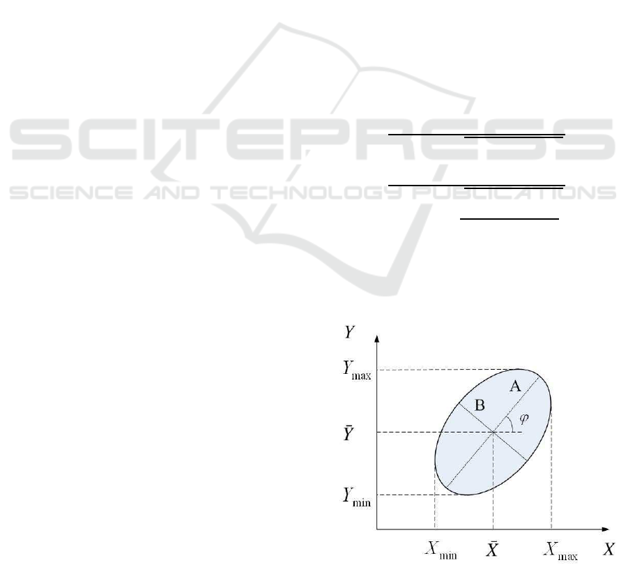
In the image plane, the ellipse is displayed in Fig.1

with its centroid, lengths of major and minor radius

and direction angle expressed in K

,i = 0,..., 5:











X = (K

−K

)/(K

−K

Y = (K

−K

)/(K

−K

2(K

+ 2K

Y + K

−K

)

+ K

−K

)

+ 4K

2(K

+ 2K

Y + K

−K

)

+ K

−

−K

)

+ 4K

E = (K

−K

)

+ 4K

)/2K

ϕ = arctan(E).

(5)

Degenerating case when projection boils down

into a segment will be avoided in the proposed path

Figure 1: Elliptical projection.

ICINCO 2016 - 13th International Conference on Informatics in Control, Automation and Robotics

planning algorithm, therefore not considered here.

Extreme values of elliptical projection in Fig.1 is

given by (Shen and Chesi, 2012b): X

max

X +

√

min

X −

√

max

Y +

√

, Y

min

Y −

√

, where µ

the central image moments of the pertinent elliptical

projection, whose centroid is calculated from raw im-

age moments m

in the form of

X = m

and

Y = m

with m

calculates the area of the el-

lipse.

Problem. The problem consists of steering an eye-in-

hand robotic arm towards the desired location follow-

ing a straight line of the camera in the Cartesian space,

with the help of some elliptical projections. Conver-

gence and FOV limit are to be imposed when features

are mainly computed from image moments of ellipti-

cal projections.

3 PATH PLANNING

Before visual servoing, a straight path of the cam-

era in the Cartesian space will be planned in advance.

Planning of this straight path needs two end positions

of the camera, this relative camera displacement is es-

timated via a virtual VS method based on image mo-

ments. However, it is not enough by only restraining

in the Cartesian space, since corresponding image tra-

jectories may go out of the image boundaries and fail

later visual servoing applications. Polynomial mini-

mization solves for the FOV problem and generates a

satisfactory trajectory by adjusting the rotational path.

The planned elliptical trajectories are then tracked by

an IBVS controller in order to follow a straight cam-

era path in the Cartesian space, at the same time with-

out losing target features.

3.1 Two Ends of a Path

Requirement of a straight path in the Cartesian space

and also camera FOV limits motivate a path-planning

method that gives a satisfactory image trajectory to

follow. Relative camera pose between the initial and

the desired positions will serve as boundaries for sub-

sequent path optimization. The target location and

model are assumed to be known as a priori and two

camera views of the target are given. From two views

of the target and an approximated camera intrinsic pa-

rameters in (1), camera pose between F

∗

and F

is es-

timated by virtually moving the camera from F

∗

to F

with a traditional IBVS controller (Tahri et al., 2010):

(t) = −λ

(s(t) −s

∗

), (6)

where T

(t) is a camera velocity screw at time t,

is a positive gain, s(t) holds the current feature

values and s

∗

the desired feature values,

is the

pseudo-inverse of the estimated interaction matrix

corresponding to the selected features. Features of a

circle is usually computed from image moments:

s = [

Y, µ

,µ

]

⊤

. (7)

As speciﬁed in Section 2,

Y are pixel coordi-

nates of the centroid of the elliptical projection. The

remaining central image moments are related to el-

lipsoid parameters in the following way (Chaumette,

1998a):

= (A

+ B

)/(1+ E

= E(A

−B

)/(1+ E

= (A

+ B

)/(1+ E

(8)

The interaction matrix associated with the fea-

ture set in (7) is referred to the work in (Chaumette,

1998a). In order to reduce the chance of local min-

imum, we will add two more features, that are pixel

coordinates of a point on the circle, to the feature set

of a circle in (7). When spheres are taken as a target,

we consider at least three spheres to reduce the possi-

bility of nonsingular occurrence of the interaction ma-

trix L. Feature set for three spheres consists of nine

values based on the computation of image moments:

s =

+µ

⊤

(9)

The associated interaction matrix may be found

in our previous work (Shen and Chesi, 2012b). The

camera position is updated iteration by iteration by

taking steps computed from velocity screw T

(t) and

time interval until feature error |s(t) − s

∗

| is small

enough. If no local minima problem exists, the ul-

timate camera position will be utilized in the subse-

quent polynomial parameterization and optimization

of the camera path.

3.2 Polynomial Minimization

To describe the camera path with boundaries on both

sides, we use a path abscise w ∈ [0,1] with its value 0

implying the start of the path F

, and value 1 meaning

the end of the path F

∗

. Transition from F

to F

∗

developed from the results in Section 3.1 and denoted

as {R,t}. Thus we have:



{R(0),t(0)}= { I

{R(1),t(1)}= { R,t} .

(10)

Between the above two camera poses, camera path

{R(w),t(w)} is intended to satisfy the FOV limits

Following a Straight Line in Visual Servoing with Elliptical Projections

when t(w) is a straight line. With path abscise w

changes from 0 to 1, camera translation t(w) linearly

changes from 0

to t, camera rotation R(w) changes

from I

to R. In between these two ends, we use

ﬁrst-order polynomials in w to model translational

path and second-order polynomials in w the rotational

quaternions:

(

q(w) = U·[w

,w, 1]

⊤

t(w) = V·[w, 1]

⊤

(11)

with

q(w) =







sin

θ(w)

a(w)

cos

θ(w)







. (12)

In quaternion representation, θ(w) ∈ (0,π) and

a(w) ∈ R

are respectively rotation angle and axis of

R(w) such that R(w) = e

θ(w)[a(w)]

Boundaries deﬁned in (10) will be satisﬁed by as-

signing the ﬁrst and last columns in the coefﬁcient

matrices in (11) with the other entries variable:











U = [ u

⊤

]

⊤

= [q−b, b,0

V = [ v

⊤

]

⊤

= [t,0

(13)

where u

⊤

∈R

1×3

, i = 1,··· ,4 are the i-th row of ma-

trix U and v

⊤

∈ R

1×2

, j = 1, 2,3 the j-th row of ma-

trix V. In (13), vector b is variable and we assign it

with an initial value of 0

. With this initial value of

b, we can plot the parameterized path for the scenario

in Fig 2 and then we have a straight path in the Carte-

sian space as shown in Fig. 3 (a). However, Fig. 3 (b)

shows that the corresponding image trajectory goes

out of the image boundary.

Therefore, we need to ﬁnd an appropriate value of

b in (13) that lets image trajectories fall within the im-

age boundaries. For a circle, depth of the circle center

is meant to be larger than the circle radius. In addi-

tion, extreme values of the elliptical projection that is

drawn in Fig. 1 are restricted to being located within

the image size:











−r > 0,

max

min

> −

max

min

> −

(14)

where X

max

, Y

max

, X

min

and Y

min

are computed from

image moments of the sphere. They are expressed as:

max

= (K

−K

)/(K

−K

min

= (K

−K

−

)/(K

−K

= (K

−K

)

−(K

−K

)(K

−K

max

= (K

−K

)/(K

−K

min

= (K

−K

−

)/(K

−K

= (K

−K

)

−(K

−K

)(K

−K

In order to realize conditions in (14), we wish to

have z

−r, X

max

, Y

max

, X

min

and Y

min

to be polynomi-

als in the path abscise w. After path parameterization,

in any camera frame of {R(w),t(w)}, we can assure

that the circle center and the normal vector in (2) are

polynomials in the path abscise. Let

⊤

]

⊤

= [0

,o] −V, (15)

which indicates h

⊤

, j = 1, 2,3 the j-th row of matrix

,o] −V, where o is the circle center in (2) and V is

coefﬁcient matrix in (11). After camera displacement

caused by varying w, polynomial coefﬁcients of the

circle center and the normal vector are computed as:

= r

∗h

+ r

∗h

+ r

∗h

= r

∗h

+ r

∗h

+ r

∗h

= r

∗h

+ r

∗h

+ r

∗h

= αr

+ βr

+ γr

= αr

+ βr

+ γr

= αr

+ βr

+ γr

(16)

where p

∈ R

and p

∈ R

, r

∈

are polynomial coefﬁcients of the entry lie in the

i-th row and the j-th column of the rotation matrix.

Speciﬁcally, we have

= u

∗u

−u

∗u

−u

∗u

+ u

∗u

= 2(u

∗u

−u

∗u

= 2(u

∗u

+ u

∗u

= 2(u

∗u

+ u

∗u

= −u

∗u

+ u

∗u

−u

∗u

+ u

∗u

= 2(u

∗u

−u

∗u

= 2(u

∗u

−u

∗u

= 2(u

∗u

+ u

∗u

= −u

∗u

−u

∗u

+ u

∗u

+ u

∗u

(17)

From equation (16), we can deduce that z

−r in

(14) is a six order polynomialin w with its coefﬁcients

to be

−r

= [0

⊤

,r] −p

. (18)

ICINCO 2016 - 13th International Conference on Informatics in Control, Automation and Robotics

Since extreme values X

max

, Y

max

, X

min

and Y

min

are

functions of K

, i = 1, ··· ,5 as given in (3.2), this for-

mulation will troubles polynomial parametrization of

these values. In order to transform inequalities in (14)

concerning these extreme values into polynomials, let

= δ

,i = 1,. .. ,5, (19)

and we will have polynomial coefﬁcients of all of k

as follows:

△

= p

∗p

+ p

∗p

+ p

∗p

−[0

⊤

= p

∗p

+ p

∗p

+ p

∗p

= p

∗p

△

+ p

∗p

−2p

∗p

= p

∗p

△

+ p

∗p

−2p

∗p

= p

∗p

△

−p

∗p

−p

∗p

= p

∗p

△

−p

∗p

−p

∗p

= p

∗p

△

−p

∗p

−p

∗p

= p

∗p

△

+ p

∗p

−2p

∗p

(20)

All of the above p

∈ R

, i = 1, ··· ,5 are poly-

nomial coefﬁcients of k

, i = 1,. .. ,5. Let

= z

−r,

= k

−k

(21)

we have ﬁrst

= (k

−k

)

−g

−k

= (k

−k

)

−g

−k

(22)

Positivity of g

and g

ensures that the maxi-

mum and minimum values of elliptical projection in

the either X or Y direction are unequal. This con-

straint avoids the degenerating case: elliptical projec-

tion boils down to a segment. Image boundary limits

are developed as follows:

= g



+ k

−k



−g

> 0,

= g



−k

+ k



−g

> 0,

= g



+ k

−k



−g

> 0,

= g



−k

+ k



−g

> 0.

(23)

Since k

, i = 1,..., 5 are polynomials, therefore g

, j =

1,··· ,7 are also polynomials in w. Their coefﬁcients

are computed from (18) and p

, i = 1, ··· ,5 in (20).

Take g

and g

for example, polynomial coefﬁcients

of g

is actually: p

= p

−r

, and coefﬁcients of g

computed as:

−k

= p

∗p

−p

∗p

−k

= p

∗p

−p

∗p

= p

∗p

−p

∗p

= p

−k

∗p

−k

−p

∗p

−k

(24)

Similar computation process applies to the polyno-

mial coefﬁcients of g

, j = 3,··· ,7. Provided the

initial value of b in (13) is given, we derive values

of U and V and bring them sequentially into (15),

(17), (16), (18) and (20). Items in (20) are utilized

in the computation of p

in (24). In order to ensure

the value of g

is positive when w ∈ (0,1), we take

the derivative of p

and solve for the corresponding

w ∈ (0,1) that give zero derivatives. If such w exist,

then a local minimum of g

can be found at such w

values. Take all of the positivity requirements of g

j = 1,··· , 7 together, we ﬁrst ﬁnd local minimums for

each g

, j = 1, ··· ,7, and again the minimum of all of

these local minimums and denote it as g

∗

= minimum

j=1

(minimum

w∈(0,1)

)),

∗

= min

(−g

∗

(25)

No action will be taken if the value of g

∗

is pos-

itive, otherwise a minimization of −g

∗

will be con-

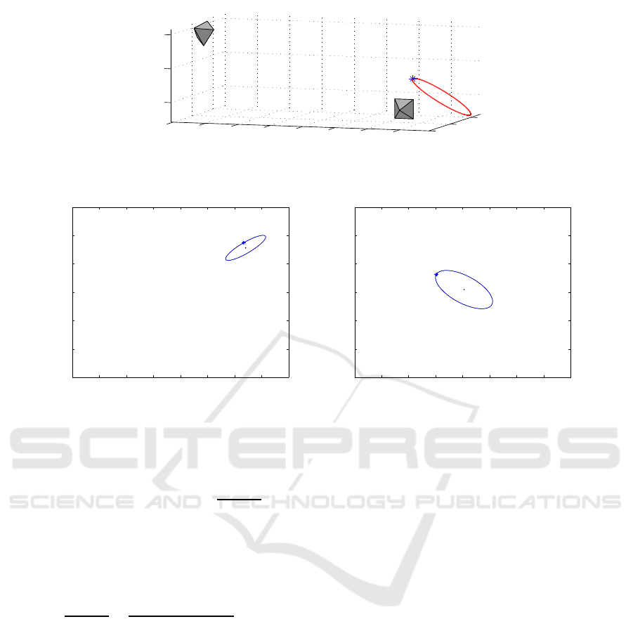
ducted until it converts its sign. Take a synthetic scene

of a circle as an example, Fig. 2 (a) consists of two

camera positions and a circle as a target. Fig. 2 (b)-

between F

∗

and F

is estimated using a virtual VS

method demonstrated in Section 3.1. A straight path

is then planned between F

∗

and F

, as shown in Fig.

3 (c). In this scenario, path planning with initial value

of b, that is 0

, will cause the image boundary vio-

lated though camera trajectory in the Cartesian space

is a straight line, see Fig. 3 (d). This situation indi-

cates that polynomial curve of g

will across below

the horizontal axis over w ∈ (0,1), and therefore g

∗

is negative. We search for appropriate value of b by

minimizing −g

∗

with MATLAB tool till g

∗

> 0. Once

the minimization result is obtained, we denote it as b

∗

and bring it into (13). Till this end, a planned path that

converges to the desired camera location following a

straight line while satisfying the camera FOV limit is

found, see Fig. 3 (e)-(f) as an example.

3.3 Tracking Image Trajectories

The robot manipulator is going to be servoed by track-

ing an well planned image trajectory. We substitute

the desired feature value s

∗

in (6) with the planned

feature value at time t, which is denoted as s

)

Following a Straight Line in Visual Servoing with Elliptical Projections

−35

−30

−25

−20

−15

−10

−5

(a)

0 100 200 300 400 500 600 700 800

100

200

300

400

500

600

(b)

0 100 200 300 400 500 600 700 800

100

200

300

400

500

600

(c)

Figure 2: Scenery with a circle and a point on the circle. (a) Scenario (b) Camera view in F

. (c) Camera view in F

∗

with w

= 1−e

−tλ

= −λ

(s(t) −s

)) + λ

∂s

)

∂t

, (26)

The term λ

∂s

)/∂t allows to compensate

the tracking error (Mezouar and Chaumette, 2002).

The partial derivative of the planned feature set is

computed as:

∂s

)

∂t

t+∆t

) −s

)

∆t

. (27)

4 EXAMPLES

The ﬁrst example aims to follow a straight line in

the Cartesian space while keeping camera FOV of a

circle. Synthetic scene is generated using MATLAB

for the ﬁrst example. The second example deals with

three Christmas balls. The algorithm keeps visibility

of all of the three balls in VS process while following

a straight line.

4.1 Simulation with a Circle

The scenario for path planning with a circle is il-

lustrated in Fig.2 (a). In the desired camera frame

of F

∗

= {I

}, model parameters of the circle are

given as [x

] = [0,0,20]

⊤

, [α,β, γ] = [0,0,1]

⊤

and r = 5mm. A point on the circle is also used to

contribute features, shown as a star mark in Fig.2 (a).

The initial and the desired camera views of the tar-

get are respectively shown in Fig.2 (b-c). From these

two views, we extract features from elliptical pro-

jections of the circle and then utilize these features

to complete planning a straight path from the initial

camera frame F

= {e

[ρ]

,[−35,10,10]

⊤

mm} with

ρ = [π/12,π/4,−π/6] to the desired camera frame

∗

. Along this straight path, the elliptical projections

of the circle are expected to be always kept within

the camera view. Intrinsic parameters of the camera

are approximated with f

= 456, f

= 448, u = 403,

v = 301 in (1).

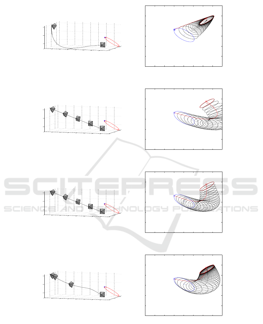
Relative camera pose between F

∗

and F

is es-

timated using a virtual VS method based on the se-

lected features. Fig. 3 (a-b) shows the camera tra-

jectory and image trajectories generated using vir-

tual VS, where the camera trajectory is extremely

close to the ground. In order to achieve the shortest

travel length, a straight path in the Cartesian space is

planned in Fig. 3 (c). With initial coefﬁcient values in

the polynomial parametrization, elliptical projections

of the circle will go beyond the image boundary and

fail a real visual servoing application, see Fig. 3 (d).

ICINCO 2016 - 13th International Conference on Informatics in Control, Automation and Robotics

−35

−30

−25

−20

−15

−10

−5

(a)

0 100 200 300 400 500 600 700 800

100

200

300

400

500

600

(b)

−35

−30

−25

−20

−15

−10

−5

(c)

0 100 200 300 400 500 600 700 800

100

200

300

400

500

600

(d)

−35

−30

−25

−20

−15

−10

−5

(e)

0 100 200 300 400 500 600 700 800

100

200

300

400

500

600

(f)

−35

−30

−25

−20

−15

−10

−5

(g)

0 100 200 300 400 500 600 700 800

100

200

300

400

500

600

(h)

Figure 3: Path planning with a circle and a point on the circle. (a) Camera trajectory in virtual IBVS. (b) Image trajectories

in virtual IBVS. (c) Planned path in workspace and camera postures without optimization. (d) Image trajectories without

optimization. (e) Planned path and camera postures in workspace. (f) Planned image trajectories. (g) Trajectory in the

Cartesian space generated when applying an IBVS controller. (h) Image trajectories generated when applying an IBVS

controller.

Following a Straight Line in Visual Servoing with Elliptical Projections

Therefore, minimization of −g

∗

in (25) is performed

to make an adjustment, after which a satisfactory im-

age trajectory is generated as shown in Fig. 3 (f). The

planned image trajectory is brought into an IBVS con-

troller in (26), where positive gains λ

, λ

and λ

are

respectively taken as 0.015, 0.01 and 0.4. An instant

camera velocity screw T

is produced and used to di-

rect the camera moving towards the desired location

by iterations. Data recorded at each iteration are plot-

ted in Fig. 3 (g)-(h).

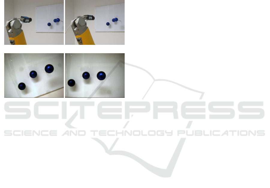
(a) (b)

Figure 4: Experiment with three Christmas balls. (a) Ini-

tial robot/camera pose. (b) Desired robot/camera pose. (c)

Initial view. (d) Desired View.

4.2 Experiment with Christmas Balls

This is a very simple experimental example validating

the proposed strategy. The robot used for the exper-

iment is a Staubli RX60 6-DoF articulated arm, on

the robot end-effector mounted a video camera. The

camera is calibrated with its intrinsic parameters as

follows:

K =





851.76868 0 329.00000

0 851.76868 246.00000

0 0 1





(28)

The target consists of three Christmas balls with

approximately the same radius of 20 mm. Positions

of these three ball centers in the desired camera frame

∗

are approximately

= [25.0183,−0.0005,344.8407]

⊤

mm,

= [−48.6174, −2.4141,412.1984]

⊤

mm,

= [−128.5265, −39.0117,414.3849]

⊤

mm.

Fig. 4 shows the two conﬁgurations and correspond-

ing camera views. Displacement between the desired

and the initial camera poses is estimated by virtual vi-

sual servoing:

R =





0.9399 0.3415 −0.0000

−0.3415 0.9399 0.0001

0.0001 −0.0001 1.0000





t = (−44.2772, −0.0353, −0.0020)

⊤

mm.

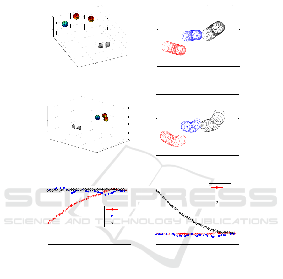
Trajectories generated in virtual VS process without

path planning are plotted in Fig. 5 (a). In virtual

VS, image trajectories of sphere centers are straight

lines, however camera trajectory is not a straight

one. After path planning and applying an IBVS con-

troller to follow the planned path, real camera tra-

jectory and image trajectories of the target are dis-

played in Fig. 5 (b)-(c), they are different from the

ones generated in virtual VS process. Iterations of

camera translation and rotation are recorded and plot-

ted in Fig. 5 (d)-(e), which show the convergence in

both camera translation and rotation. It is assumed

that iteration number in real-time step-by-step mov-

ing robotic application is denoted as t, trajectories

(t) = [q

(t),q

(t)]

⊤

in Fig. 5 (e) are Cayley

representation (Craig, 2005) of the associated rotation

matrix R(t):

(t)]

= (R(t) −I

)(R(t) + I

)

−1

. (29)

Fluctuations exist in the iterations mainly due to

coarse feature extraction and the value of tracking

gain used for computing the next arriving position in

VS process for the step-by-step moving robot.

5 CONCLUSIONS

This paper proposes a straight path planning approach

for visual servoing with elliptical projections. Cir-

cles and spheres may project into traditional cameras

as ellipsoids. Constrains with spheres are considered

in our previous work, this paper mainly solves for

problems with circular objects, speciﬁcally the con-

vergence and FOV limit while following a straight

line in the Cartesian space. Simulation with a cir-

cle and experiment with balls validate the proposed

path planning approach. For future work, the impact

of image noises imported from the area-based feature

extraction on the precision of pose estimation and the

subsequent path planning needs to be taken case of.

More complicated objects are going to be explored,

such as a cup to be seen as a group of two lines or two

circles.

ICINCO 2016 - 13th International Conference on Informatics in Control, Automation and Robotics

−200

−100

100

200

300

−100

−50

x [mm]

z [mm]

y [mm]

0 100 200 300 400 500 600

100

200

300

400

[pixel]

(a)

−200

200

400

−100

100

z [mm]

x [mm]

y [mm]

(b)

0 100 200 300 400 500 600

100

200

300

400

[pixel]

(c)

0 5 10 15 20 25 30 35

−10

−8

−6

−4

−2

iteration

translation [cm]

(d)

0 5 10 15 20 25 30 35

−5

iteration

rotation [deg]

(e)

Figure 5: Experiment with three Christmas balls. (a) Virtual Camera path. (b) Virtual image trajectories. (c) Real camera

path. (d) Real image trajectories. (e) Camera translation evolution. (f) Camera rotation evolution.

REFERENCES

Chaumette, F. (1998a). De la perception `a l’action:

l’asservissement visuel; de l’action `a la perception:

la vision active. Habilitation `a diriger les recherches,

Universit´e de Rennes 1.

Chaumette, F. (1998b). Potential problems of stability and

convergence in image-based and position-based visual

servoing. In Kriegman, D., Hager, G., and Morse,

A. S., editors, The Conﬂuence of Vision and Control,

pages 66–78. LNCIS Series, No 237, Springer-Verlag.

Chaumette, F. (2004). Image moments: a general and useful

set of features for visual servoing. IEEE Transactions

on Robotics, 20(4):713–723.

Chaumette, F. and Hutchinson, S. (2006). Visual servo con-

trol, part I: Basic approaches. IEEE Robotics and Au-

tomation Magazine, 13(4):82–90.

Chaumette, F. and Hutchinson, S. (2007). Visual servo con-

trol, part II: Advanced approaches. IEEE Robotics and

Automation Magazine, 14(1):109–118.

Chesi, G. and Hashimoto, K., editors (2010). Visual Ser-

voing via Advanced Numerical Methods. Springer-

Verlag.

Chesi, G., Hashimoto, K., Prattichizzo, D., and Vicino, A.

(2004). Keeping features in the ﬁeld of view in eye-

in-hand visual servoing: A switching approach. IEEE

Transactions on Robotics, 20(5):908–914.

Collewet, C. and Marchand, E. (2010). Luminance: a

new visual feature for visual servoing. In Chesi, G.

and Hashimotos, K., editors, Visual Servoing via Ad-

Following a Straight Line in Visual Servoing with Elliptical Projections

vanced Numerical Methods, pages 71–90. LNCIS Se-

ries, No 401, Springer-Verlag.

Cowan, N., Weingarten, J., and Koditschek, D. (2002). Vi-

sual servoing via navigation functions. IEEE Trans-

actions on Robotics and Automation, 18(4):521–533.

Craig, J. J. (2005). Introduction to Robotics: Mechanics

and Control. Pearson Education, 3rd edition.

Fomena, R. T. and Chaumette, F. (2008). Visual servoing

from two special compounds of features using a spher-

ical projection model. In IROS’08, 21st IEEE/RSJ In-

ternational Conference on Intelligent Robots and Sys-

tems, pages 3040–3045, Nice, France.

Gans, N. and Hutchinson, S. (2007). Stable visual servoing

through hybrid switched-system control. IEEE Trans-

actions on Robotics, 23(3):530–540.

Hashimoto, K., Kimoto, T., Ebine, T., and Kimura, H.

(1991). Manipulator control with image-based visual

servo. In ICRA’91, 8th IEEE International Confer-

ence on Robotics and Automation, pages 2267–2272,

San Francisco, CA.

Malis, E., Chaumette, F., and Boudet, S. (1999). 2 1/2 d

visual servoing. IEEE Transactions on Robotics and

Automation, 15(2):238–250.

Mezouar, Y. and Chaumette, F. (2002). Path planning for

robust image-based control. IEEE Transactions on

Robotics and Automation, 18(4):534–549.

Oh, P. Y. and Allen, P. K. (2001). Visual servoing by par-

titioning degrees of freedom. IEEE Transactions on

Robotics and Automation, 17(1):1–17.

Shen, T. and Chesi, G. (2012a). Visual servoing path-

planning for cameras obeying the uniﬁed model. Ad-

vanced Robotics, 26(8–9):843–860.

Shen, T. and Chesi, G. (2012b). Visual servoing path-

planning with spheres. In ICINCO’12, 9th Interna-

tional Conference on Informatics in Control, Automa-

tion and Robotics, pages 22–30, Rome, Italy.

Shen, T., Radmard, S., Chan, A., Croft, E. A., and Chesi,

G. (2013). Motion planning from demonstrations and

polynomial optimization for visual servoing applica-

tions. In IROS’13, 26th IEEE/RSJ International Con-

ference on Intelligent Robots and Systems, pages 578–

583, Tokyo Big Sight, Japan.

Tahri, O., Araujo, H., Chaumette, F., and Mezouar, Y.

(2013). Robust image-based visual servoing using in-

variant visual information. Robotics and Autonomous

Systems, 61(12):1588–1600.

Tahri, O. and Chaumette, F. (2005). Point-based and region-

based image moments for visual servoing of planar

objects. IEEE Transactions on Robotics, 21(6):1116–

1127.

Tahri, O., Mezouar, Y., Chaumette, F., and Araujo, H.

(2010). Visual servoing and pose estimation with

cameras obeying the uniﬁed model. In Chesi, G.

and Hashimotos, K., editors, Visual Servoing via Ad-

vanced Numerical Methods, pages 231–252. LNCIS

Series, No 401, Springer-Verlag.

Taylor, C. and Ostrowski, J. (2000). Robust vision-based

pose control. In ICRA’00, 17th IEEE International

Conference on Robotics and Automation, pages 2734–

2740, San Francisco, CA.

ICINCO 2016 - 13th International Conference on Informatics in Control, Automation and Robotics