
Occupancy Grid Mapping with Highly Uncertain Range Sensors based
on Inverse Particle Filters
Timo Korthals, Marvin Barther, Thomas Sch
¨
opping, Stefan Herbrechtsmeier and Ulrich R
¨
uckert
Cognitronics & Sensor Systems, Bielefeld University, Inspiration 1, 33619 Bielefeld, Germany
Keywords:
Occupancy Grid Mapping, Inverse Sensor Model, Inverse Particle Filter, Uncertain Range Sensors.
Abstract:
A huge number of techniques for detecting and mapping obstacles based on LIDAR and SONAR exist, though
not taking approximative sensors with high levels of uncertainty into consideration. The proposed mapping
method in this article is undertaken by detecting surfaces and approximating objects by distance using sensors
with high localization ambiguity. Detection is based on an Inverse Particle Filter, which uses readings from
single or multiple sensors as well as a robot’s motion. This contribution describes the extension of the Sequen-
tial Importance Resampling filter to detect objects based on an analytical sensor model and embedding into
Occupancy Grid Maps. The approach has been applied to the autonomous mini robot AMiRo in a distributed
way. There were promising results for its low-power, low-cost proximity sensors in various real life mapping
scenarios, which outperform the standard Inverse Sensor Model approach.
1 INTRODUCTION
Static obstacle detection for robotic systems is a well-
known and commonly studied scientific field (Thrun,
2002; Thrun, 2003; H
¨
ahnel, 2004). It is a part of ev-
ery local collision avoidance system set up to maneu-
ver through cluttered environments. Another impor-
tant application is the creation of obstacle maps while
traversing an unknown area and the recognition of al-
ready known obstacles, so supporting the localization.
In nowadays robotic applications most mapping
challenges are commonly faced by applying the best
sensor for the job, which is a high accurate laser range
finder in case of a mapping and localization task.
These challenges mostly involve high setup costs and
therefore low-cost sensors with high measurement un-
certainties tend to get disregarded when it comes to
algorithm design. However, these kind of sensors still
make their way into mini and swarm robots, which
are used for educational and research applications that
demand low-cost and highly redundant setups. With
today’s developments in microelectronic technology,
small sized robots can be built with all the functional
properties of full sized robots but with the added ben-
efits of affordability, economy of space, and fast setup
time. These platforms offer a solution for carrying out
real life robotics, besides simulation, on a large scale
and in a cost efficient way (Navarro and Mat
´
ıa, 2013).
In an attempt to lower costs, hardware designers
tends to integrate sensors that may not fulfill today’s
accuracy requirements for mapping and localization.
High uncertainty proximity sensors play a significant
role in these cases. They are highly integrable and
very cheap but are disadvantaged by their poor range
and angle resolution. Despite this, they are commonly
used for basic collision avoiding behaviors.
Our contribution overcomes the disadvantages of
high ambiguity sensors by proposing an Inverse Par-
ticle Filter design, which directly samples from the
analytical Inverse Sensor Model to retrieve a refined
assumption of static objects in the robotics’ surround-
ings. The particles themselves are then modeled as an
Inverse Sensor Model for Occupancy Grid Mapping,
which results can then directly be used for planning
and navigation algorithms in situations that demand a
global representation of the environment.
This paper is organized as follows: Section 2 high-
lights the different sensor techniques that are used for
Occupancy Grid Mapping, where we also define the
radiation based proximity sensor. In Section 3, we
describe the design of our Inverse Particle Filter ap-
proach to a general proximity sensor model and the
extension to an Inverse Sensor Model for an Occu-
pancy Grid Map algorithm. Recommended imple-
mentation of our application is provided in Section 4.
Finally, in Section 5 we explain and reflect on our var-
ious evaluations, and offer conclusions of our work in
Section 6.
192
Korthals, T., Barther, M., Schöpping, T., Herbrechtsmeier, S. and Rückert, U.
Occupancy Grid Mapping with Highly Uncertain Range Sensors based on Inverse Particle Filters.
DOI: 10.5220/0005960001920200
In Proceedings of the 13th International Conference on Informatics in Control, Automation and Robotics (ICINCO 2016) - Volume 2, pages 192-200
ISBN: 978-989-758-198-4
Copyright
c
2016 by SCITEPRESS – Science and Technology Publications, Lda. All rights reserved
2 SENSORS FOR MAPPING
To realize Occupancy Grid Mapping, sensor readings
are interpreted via the Inverse Sensor Model which
allows the reasoning from the measurement to the ac-
tual distance of a given object (Thrun, 2002). Laser
range finders and ultrasonic sensors are commonly
used to acquire information about distance. This in-
formation can then be mapped onto the robot’s envi-
ronment model to build up its view of its surround-
ings.
2.1 Comparison of Sensors
The laser range finder is the most convenient sensor,
as it can perform a range measurement by sending
out a single ray of light. Via modulation or time-of-
flight techniques, the distance of a single distinctive
spot can be determined with high precision. While
it is a state-of-the-art sensor for any range detection,
there are also numerous drawbacks to it, namely high
power consumption, mechanical parts, and high setup
costs.
An ultrasonic based sensor measures distance by
time-of-flight, sending out an ultrasonic wave, which
is reflected and then detected for a second time. In the
history of robotic applications, this sensor was one of
the first for mapping and localization tasks, and has
therefore been well studied (Thrun, 2002; Moravec
and Elfes, 1985). The numerous disadvantages of the
high ambiguity sensor lobes and the influences of an
object’s surface, distance, shape, reflectance and abra-
siveness make this sensor relatively outdated for tasks
today. Additionally, the sensor’s large physical di-
mensions and price makes it useless it for small and
highly integrated robots (cf. Table 1).
Proximity sensors are commonly infrared based
diode pairs, consisting of an emitting light source
where the reflected intensity is measured over a cer-
tain period of time via a photo diode. The significant
advantage of these kinds of sensors is their high inte-
grability into electric circuits due their small housing.
The small measurement range of a few decimeters is
negligible due to the operational scenarios in mini-
and swarm robots with a footprint less than 100 cm
3
(Navarro and Mat
´
ıa, 2013). On the other hand, the
high ambiguity sensor lobe makes it apparently im-
possible to apply proximity sensors in mapping appli-
cations.
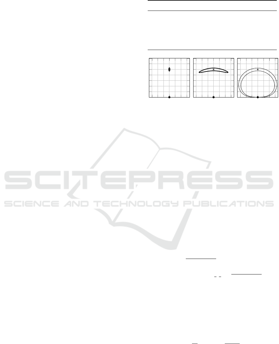
Figure 1 qualitatively shows the different sensor
lobes that are used in Occupancy Grid Mapping. This
top view is a hypothetical obstacle measurement in
the sensor frame. For each sensor, the uncertainty of
the objects localization is visualized by the standard
Table 1: Feature comparison of range sensors in robotics.
Laser Sonar Proximity
Volume (cm
3
) > 175 ∼ 12 ∼ 0.01
Range (m) > 10 < 5 < 0.5
Powerdraw (mW) > 250 < 100 < 50
Precision (%) ∼ 1 ∼ 10 ∼ 10
Price ($) > 100 ∼ 10 ∼ 1
(a) LIDAR (b) SONAR (c) Proximity
Figure 1:
·
: Sensor position, x: Obstacle, -: Standard error
contour of qualitative sensor cones at full range.
error contour by range and angular resolution.
2.2 Analytical Sensor Model
For our scenario, we use a radiation based proximity
sensor which approximately follows the photometry
inverse square law s(x,Θ) = α
i
α
0
cosΘ/x
2
+β (Benet
et al., 2002). Θ is the angle of incidence while x is the
distance between sensor and object. The model’s pa-
rameters can be interpreted as follows: α
0
is constant
and describes the radiant intensity of the emitter, the
spectral sensitivity of the receiver, and the gain of the
internal amplifier. α
i
depends on the object’s surface
and represents the reflectivity constant. β is the off-
set value that remains, whenever there is no object in
range. The Inverse Sensor Model, s.t. determining the
distance x from the measured value s is
s(x,Θ) =
α
i
α
0
cos(Θ)
x
2
+ β
⇒ x
2
(s)
Θ∈
[
−
π
2
,
π
2
]
=
α
i
α
0
cos(Θ)
s −β
.
The disadvantage of the Inverse Sensor Model is the
ambiguity of an object’s position over the angle Θ and
distance x (cf. Figure 1). Additionally, we introduce
sensor noise σ
s
which we assume to be Gaussian and
constant over the angle Θ. The error propagation for
the resulting distance uncertainty σ
x
can be calculated
as follows:
σ
x
=
∂x
∂s
Θ=0
σ
s
=
x
2α
i
α
0
σ
s
.
The resulting standard error of a measured object with
different distances to the sensor shown qualitatively in
Figure 1.
Occupancy Grid Mapping with Highly Uncertain Range Sensors based on Inverse Particle Filters
193
2.3 Occupancy Grid Mapping
Elfes introduces the two dimensional Occupancy Grid
Map (OGM) (Elfes, 1989). This representation sub-
divides the planar environment into a regular array
of rectangular cells. Each cell represents a static lo-
cation, comprising information on the covered area.
Thus, the resolution of the environment representa-
tion directly depends on the size of the cells. In
addition to this discretization of space, a probabilis-
tic measure regarding state is associated with each
cell. In terms of robotic navigation and mapping, this
state represents space occupancy, while the mapping
of other features has also been studied by the author
(Korthals et al., 2015).
H
¨
ahnel states that measurements take on any real
number in the interval [0,1] and describes one of two
possible cell states: occupied or free. The occupancy
probability of 0 means that there is definitely free
space, the probability of 1 means that there is def-
initely occupied space and a value of 0.5 refers to
an unknown state of being occupied (H
¨
ahnel, 2004).
Many methods have been employed in updating the
state of occupancy for each cell, such as Bayesian
(Matthies and Elfes, 1988; Elfes, 1992), Dempster-
Shafer (Carlson and Murphy, 2005), and Fuzzy Logic
(Plascencia and Bendtsen, 2009).
A probabilistic Inverse Sensor Model (ISM) is
used to update the OGM in a Bayesian framework,
which deduces the occupancy probability of a cell,
given its sensor measurement. The technique to de-
rive models for LIDAR and SONAR sensors have
been well studied by Thrun (Thrun et al., 2005),
H
¨
ahnel (H
¨
ahnel, 2004), and Stachniss (Stachniss,
2009). We adopted the ISM from Stanchniss and
H
¨
ahnel for proximity sensors as depicted in Figure 2.
3 INVERTED PARTICLE FILTER
Particle filters are commonly used to find the posi-
tion of a robot based on measurements of its environ-
ment. The Inverse Particle Filter (IPF) described in
this section inverts the problem: It finds the position
of the environment based on measurements from its
position. The output from the IPF is therefore an esti-
mate, based on each particle, of the surfaces of objects
surrounding the robot.
In order to update the IPF and global OGM, the
robot needs two representations of its environment:
First, the IPF resides in a local circular map with the
robot in its center. Second, the OGM is a global map
with a fixed coordinate system in space, which can
be traversed by the robot. As the robot moves, each
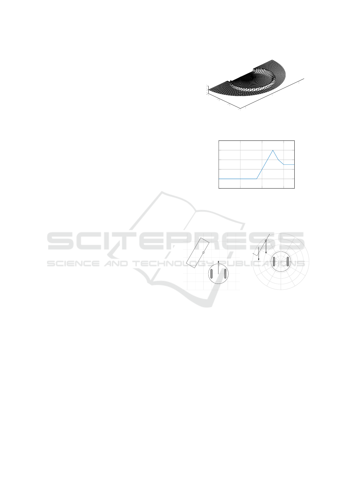
0
2
4
6
−5
0
5
0
0.5
1
Distance (cm)
Distance (cm)
Occupancy Probability
(a) Planar occupancy probability
0 2 4
6
0
0.2
0.4
0.6
0.8
1
Distance (cm)
Occupancy Probability
(b) Occupancy probability along radial axis
Figure 2: Inverse Sensor Model for radiation based proxim-
ity sensors measuring an object at 5 cm.
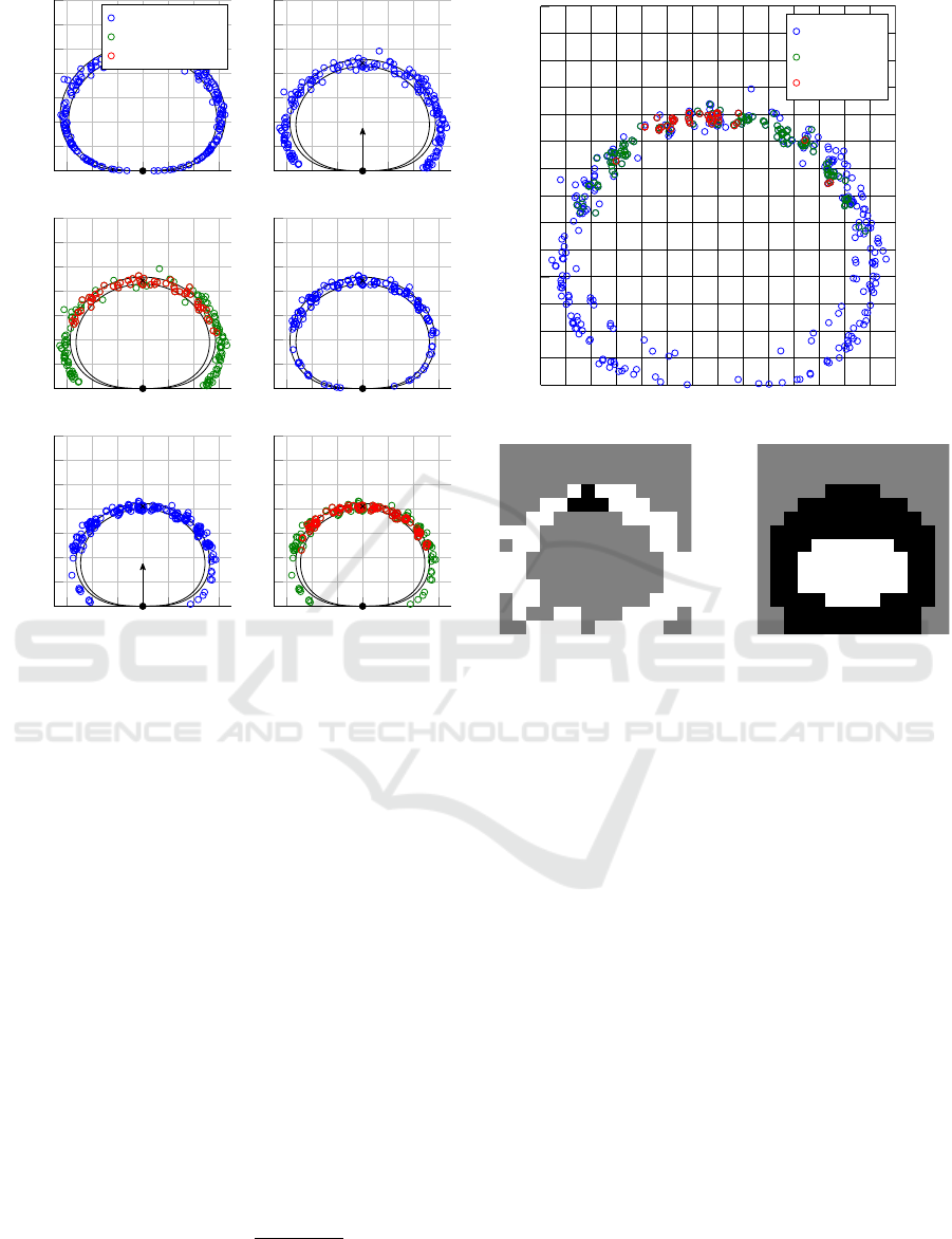
u
Object Contour
Particle
(a) Global frame
−u
Object Contour
Particle
−u
(b) Local frame
Figure 3: Locomotion of robot and objects for steering com-
mand u.
particle in the local map will move in the opposite di-
rection respectively. This reflects the position of the
particle relative to the new position of the robot, as
shown in Figure 3(b). In the OGM frame, shown
in Figure 3(a), the situation is reversed, where each
sampled particle remains in position and represents a
static object in space.
For our initial work, we used the IPF technique ap-
proach as proposed by Kleppe (Kleppe and Skavhaug,
2013). Kleppe applied the IPF to a single laser range
finding application that was mounted on a mini robot
with restricted movement. In the following sections,
we accommodate his work and extend the IPF in three
ways: First, we use a full analytical model of the sen-
sor instead of heuristics to make the IPF generally
valid. Second, the extension to a multi sensor setup
ICINCO 2016 - 13th International Conference on Informatics in Control, Automation and Robotics
194

Table 2: Variables used in the SIR filter.
I Number of particles
{
·
}
I
i=1
Feature set of I particles
k Particle position in local frame
t Time step
w Weight of a particle
e Epoch counter
z Sensor measurement
u Steering command
p(p|k, u) Error model of the inverse kinematic
p(z|k) PDF of the analytical ISM
is proposed and third, we finalize our IPF with an un-
derlying OGM, so that our approach can be directly
fed into any common robotic navigation application.
3.1 Inverse Particle Filter
To accomplish the objects’ localization from the read-
ings, we must use the Sequential Importance Resam-
pling (SIR) filter as described in Algorithm 1 with
the variables from Table 2. First, the Inverse Kine-
matic Model (IKM) is applied to the old set
{
·
}
I
i=1
of particles. The IKM is the relative movement of
the particles in the robots frame with the respective
error model. A detailed description is given in Sec-
tion 4.4 for a robot with differential kinematic. Sec-
ond, the score of each particle, that being an objects
surface representation, is calculated by evaluating the
new ISM at each particle position.
Algorithm 1: SIR-Filter.
Require:
{
k
t−1
,w
t−1
,e
t−1
}
I
i=1
,z
t
,u
t
1: for all k
t−1
in range do
2: ˜p
(i)
t
∼ p(p
t
|k
(i)
t−1
,u
t
) Apply IKM
3: ˜w
(i)
t
= p(z
t
|k
(i)
t
) Apply ISM
4: end for
5: for all ˜w
t
do
6: w
t
= Normalize( ˜w
t
)
7: end for
8: for all k
t
do
9: k
t
= Resample(w
t
)
10: e
t
= e
t
+ 1
11: end for
Ensure:
{
k
t
,w
t
}
I
i=1
A new aspect in our SIR filter can be found by
counting the particles’ survived epochs e. This value
is used for Innovation Gating (IG) in the OGM, where
only particles are taken as true obstacle estimations
if the epoch counter is greater than a certain gating
value.
To ensure fast convergence, we do not generate
new samples randomly, but directly from the ISM via
Algorithm 2. If we want to find the hidden distribu-
tion of obstacles in the environment , then ISM gives
us the best approximation of the unknown distribu-
tion. N denotes the number of sensors attached to the
robot, and s
t
the measured value of sensor n at time t.
Algorithm 2: Generation of new Particles.
Require:
{
s
t
}
N
n=1
1: ˜n ∼ U(1,N) Draw a sensor
2:
˜
φ ∼ U(−90
◦
,90
◦
) Draw a local angle
3: ˜r ∼ N (s
n
,σ
s
n
) Draw a local distance to the
sensor
4: x
t
=
˜r,
˜
φ
Ensure: k
t
An example of two IPF steps can be seen in Fig-
ure 4. At t = 0, an initial measurement of an object
that is 10 cm in front of the sensor is received. Thus,
the IPF is bootstrapped, drawing 100 % of particles,
s.t. object hypothesis, from the sensor model. Next,
the sensor moves towards the object which results in
the relative motion for all particles and the object in
the sensor frame. Here, the IKM is applied to every
particle. In Figure 4(c), a score is calculated for ev-
ery particle based on the current measurement. 80 %
of particles survive this epoch, while the remaining
20 % are rejected and sampled from the current sensor
model. At t = 2, a consecutive motion and importance
resampling is applied again.
The movement u
t
is a very significant feature for
acquiring the objects’ positions from the ambiguous
sensor readings z
t
, due to the fact that the history of
sensor readings is strongly correlated to the real ob-
jects’ positions. The movement and error propagation
of the particle is derived for a differential kinematic in
Section 4.4. It also affects the sampling frequency of
the IPF itself so that we introduce a sample-per-speed
ratio SSR with
[SSR] =
IPF Sample Frequency
Linear Vehicle Velocity
=
Hz
m/s
(1)
which has to remain constant at any time to ensure
functionality of the IPF. If this cannot be guaranteed,
e.g., if the robot stands still, the IPF needs to be tem-
porarily switched off. Otherwise, it would find ran-
dom objects based on sensor noise.
To respect more than one sensor via the IPF, we
can extend the calculation to weights of each particle.
The overall weight w
t,N
results from evaluating each
ISM of N sensors at the particles position in the local
frame. The derived probabilities are then fused by De
Morgan’s law as follows:
w
t,N
= P(x
t
|s
t
) = 1 −
N
∏
n=1
1 −P(x
t
|s
t,n
). (2)
Occupancy Grid Mapping with Highly Uncertain Range Sensors based on Inverse Particle Filters
195
-.06 -.04 -.02 0 .02 .04 .06
0
.02
.04
.06
.08
.1
.12
.14
Distance (m)
Surface Hypothesis
Rejected
Survived
(a) t = 0: Sampling 100 %
-.06 -.04 -.02 0 .02 .04 .06
0
.02
.04
.06
.08
.1
.12
.14
u
(b) t = 1: Translation
-.06 -.04 -.02 0 .02 .04 .06
0
.02
.04
.06
.08
.1
.12
.14
Distance (m)
(c) t = 1: Resampling
-.06 -.04 -.02 0 .02 .04 .06
0
.02
.04
.06
.08
.1
.12
.14
(d) t = 1: Sampling 20 %
-.06 -.04 -.02 0 .02 .04 .06
0
.02
.04
.06
.08
.1
.12
.14
Distance (m)
Distance (m)
u
(e) t = 2: Translation
-.06 -.04 -.02 0 .02 .04 .06
0
.02
.04
.06
.08
.1
.12
.14
Distance (m)
(f) t = 1: Resampling
Figure 4: Two steps of the SIR-Filter depicted line-wise
from top-left to bottom-right in the sensor frame.
·
: Sensor
position, x: Obstacle, -: Standard error contour.
3.2 Learning Occupancy Grid Maps
Our new approach updates a cell c =
{
c
free
,c
occ
}
in
the map by interpreting each particle falling within
this cell as follows:
c
free
+ 1 , if i was rejected,
c
occ
+ 1 , if i survived and e
i
≥ g,
back off , if i survived and e
i
< g.
(3)
Every resampled particle k
i
that was rejected for the
next epoch is taken as free space since it does not
match the surface estimate of a wall. On the other
hand, all sampled particles surviving the epoch are
interpreted as occupied, taking IG into account. Par-
ticles that haven’t survived the necessary amount of
epochs are backed off and do not increase c
free
nor
c
focc
. Finally, the state of a cell is calculated by ap-
plying the counting model (H
¨
ahnel, 2004):
f
occ
(c
occ
,c
free
) =
c
occ
c
occ
+ c
free
.
(4)
Figure 5 shows the result of sorting the particles
(cf. Figure 5(a)) from the steps depicted in Figure 4
-.06 -.04 -.02 0 .02 .04 .06
0
.02
.04
.06
.08
.1
.12
.14
Rejected
e = 1
e = 2
(a) Particles in global frame
(b) IPF in OGM (c) ISM in OGM
Figure 5: OGM comparison between IPF and ISM.
into an OGM (cf. Figure 5(b)). The OGM reference
frame is a fixed global one and coincides with the ini-
tial sensor position at t = 0. Figure 5(a) shows the sur-
vived and rejected particles in the initial sensor frame
at t = 0 with an overlaid discretization. The corre-
sponding OGM is deduced by applying the rules from
Equation 3 and Equation 4 with g = 2. Figure 5(c)
shows the same OGM but created by the standard ISM
derived from the analytical sensor model.
4 IMPLEMENTATION
We implemented and tested our Inverse Sensor Model
approach on the Autonomous Mini Robot (AMiRo).
Section 4.1 briefly describes the robot itself and its
hardware. Our approach is depicted in Section 4.2.
Finally, the analytical sensor model for the robots
proximity sensors is analyzed and optimized in Sec-
tion 4.3.
4.1 AMiRo
As can be seen in Figure 6(a), AMiRo was developed
ICINCO 2016 - 13th International Conference on Informatics in Control, Automation and Robotics
196

(a) AMiRo (b) Footprint
Figure 6: AMiRo platform with footprint of kinematic and
its eight co-circular arranged proximity sensors (4).
by Herbrechtmeier et. al. (Herbrechtsmeier et al.,
2012) at the Cogitive Interaction Technology - Cen-
ter of Excellence (University of Bielefeld, Germany).
The robot has a cylindrical shape with a diameter of
100 mm and a height of 76 mm. Two wheels give
the ability for locomotion through differential steer-
ing. Our setup of the AMiRo consists of three differ-
ent modules, each of which has been designed to han-
dle specific tasks: DiWheelDrive (STM32F103 MCU
for motion control and odometry), PowerManage-
ment (STM32F405 MCU for object recognition, and
basic behavior), Cognition (DM3730 SoC for high-
level planning tasks and WLAN communication). In
order to permit the mapping task, PowerManagement
is extended by eight integrated sensors, arranged as
depicted in Figure 6(b) for proximity measurements.
4.2 Realization
Our approach is implemented on the AMs in a dis-
tributed fashion. The IPF, s.t. the periodic sam-
pling of distant surfaces, strongly demands a real-
time approach to ensure that all samples and particle
weights are calculated before a new sensor measure-
ment arrives. Thus, this part was carried out on the
PowerManagement AM. Another important aspect of
our approach is the fact, that the quality of sampling
strongly depended on driving distance (see Section 3).
This is satisfied by keeping the SSR constant via su-
persampling the sensors at 125 Hz and downsampling
to any requested rate.
The mapping, s.t. the sorting of the particles into
an array structure, is a highly memory consuming
application with respect to the limited hardware re-
sources on the robot. Though not mandatory, it also
requires dynamic allocatable memory to extend map
dimensions on demand. Therefore, it is unfeasible for
it to be realized in a real-time fashion on the MCU
based boards and thus become implemented on the
Cognition AM.
For evaluation, the Cognition AM logs all steer-
ing, localization and sensor messages. Afterwards,
we analyze, evaluate, and prove our approach via a
MATLAB based implementation.
4.3 Optimized Sensor Model
For our proximity sensor, we chose the integrated
infrared based proximity sensors VCNL4020 by
Vishay, which only approximately follows the pho-
tometry inverse square law as described by Benet et
al. (Benet et al., 2002). The maximum range of the
sensors x
max
is about 20 cm, while the maximum an-
gle of incidence θ
max
is at 60
◦
.
For the correction of the cone characteristic the
constant ξ has been added to modulate the cosine. Ad-
ditionally, the constant α depends on the distance of
the object. This behavior originates from the fact that
if the object were to be closer to the sensor, the re-
flecting ground area would also decrease. Thus, the
constant α is extended by a linear function in depen-
dence of its sensor value. Finally the advanced sensor
model is defined as:
x
2
(s,Θ) =
α
i
α
0
cos(ξΘ)
s −β
+ δcos(ξΘ),
σ
x
(x,Θ) =
x
2
cos(ξ·Θ)
−δ
2
2
√
cos(ξ·Θ)
α
i
α
0
x
σ
s
.
(5)
The ISM x(s,Θ) and error model σ
x
(x,Θ) from Equa-
tion 5 are used by the IPF in our evaluation scenario.
4.4 Inverse Kinematic Model
Since the IPF resides in the robot frame, the robot
does not move by the steering command u, but
rather each particle respectively. The vehicles veloc-
ities
v
x
,v
y
,ω
in the global planar frame are deter-
mined using a differential kinematic’s steering com-
mands u = (v
l
,v
r
), as illustrated in Figure 3, and the
basewidth b after the Euler method as shown in Equa-
tion 6. Further, we can omit the robot’s orientation Θ
since we are only interested in the particles’ velocities
in each step in the robot’s frame
v
x
v
y
ω
Θ=0
=
1
/2(v
l
+ v
r
)
0
1
/b(v
l
−v
r
)
. (6)
From Equation 6, the relative particle motion denoted
by “P” in the vehicle frame at position (r,θ) can be
written as follows:
v
P,x
v
P,y
=
v
l
+v
r
2
−
v
l
−v
r
b
r sin(φ)
−
v
l
−v
r
b
r cos(φ)
. (7)
The particle’s next position, F, can now be directly
derived from Equation 7:
F =
x
t+1
y
t+1
=
x
t
+ ∆t ·v
P,x
y
t
+ ∆t ·v
P,y
. (8)
Occupancy Grid Mapping with Highly Uncertain Range Sensors based on Inverse Particle Filters
197
Assuming Gaussian uncertainty for each particle, one
can now derive error propagation from Equation 8 by
calculating the Jacobian J
F
of F. The resulting model
can be directly applied as IKM in Algorithm 1.
5 EVALUATION
We evaluated various mapping scenarios to bench-
mark our approach in the individual situations (cf.
Figure 7). All objects consist out of acrylic blocks
with the dimensions 200 mm x 50 mm x 70 mm.
Therefore, we decided that every object construction
should be at least of the same dimensions of the robot.
The robot drives with 80 mm/s, while the sensor fre-
quency is 8 Hz. Thus, by applying Equation 1, we
gain a SSR of 0.1 Hz per mm/s.
Quantitative benchmarking is carried out by eval-
uating the resulting OGM after path traversal against
a deduced map by an adapted ISM for sonar sensors,
as described in Section 2.3. We calculate the Over-
all Mapping Errors (OE) with respect to the Ground
Truth (GT) map as proposed by Carvalho (Carvalho
and Ventura, 2013):
OE =
# False Positives + # False Negatives
# All Classified Cells
. (9)
For benchmarking, we decided to expand the walls
by a maximum of half the robots radius for bench-
marking. This was done because measurements of a
proximity sensor are not absolutely accurate, as the
name suggests. But common navigation algorithms
for OGMs expand all found walls by at least half of
the robots radius anyway. Thus, we take the best OE
value within this range.
The chosen scores do not fully comprise the qual-
ity of the deduced OGMs. It is not really beneficial
compare the standard ISM against the IPF of the full
driven paths, as it is not known how the algorithms
will perform in between. This is important for nav-
igation and obstacle avoidance algorithms that must
perform the path traversal on the OGM.
5.1 Scenario Description
In the Single Sensor - Single Object (SSSO) sce-
nario, a single block is placed horizontally in front of
a sensor. The robot approaches the short side of the
block. It starts at a distance of 350 mm to the block
and approaches it until it is 60 mm away. The Multi-
ple Sensors - Single Object (MSSO) scenario is the
same as the SSSO, but with all eight sensors activated.
For the Multiple Sensors - Object Drive-by
(MSOD) scenario, a single block is placed horizon-
tally beside the robot. The robot drives along the
0 .05 .1 .15 .2 .25 .3 .35 .4
-.05
0
.05
Distance (m)
Distance (m)
Start
End
(a) Single Object
0 .1 .2 .3 .4 .5 .6
.7
.8
-.1
-.05
0
.05
.1
.15
Distance (m)
Distance (m)
(b) Drive-by
0 .2 .4 .6
0
.2
.4
.6
.8
1
Distance (m)
Distance (m)
(c) L
0 .2 .4 .6
0
.2
.4
.6
.8
1
Distance (m)
(d) T
Figure 7: Ground Truth scenarios.
long side of the block at a constant surface distance
of 100 mm with all sensors activated. In the Multiple
Sensors - Maze (MSM) scenarios, multiple blocks
are arranged in L- and T-shape mazes. Within the
navigation task, the robot is required to drive on a pre-
defined trajectory with all sensors activated.
5.2 Benchmark
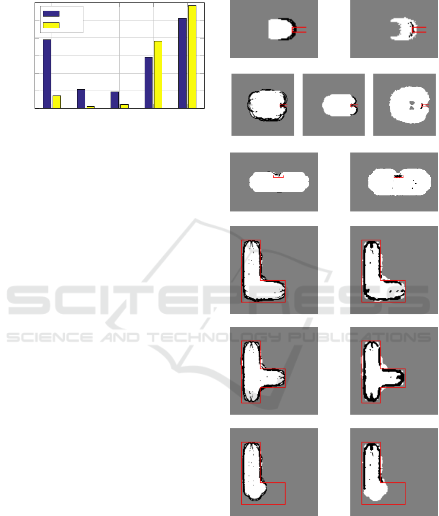
Figure 9 shows different OGM mappings of the ISM
in comparison to the new proposed IPF. The OGMs
are visualized, such that white space denotes values
f
occ
< 0.5, black space f
occ
> 0.5, and grey space (s.t.
unknown, with no readings acquired yet) f
occ
= 0.5.
The red shape is the obstacles GT overlay. All IPF
related OGMs are deduced with g = 4 and 1000 par-
ticles per sensor.
Figure 9(a) and Figure 9(b) show the real outcome
for the artificial scenario depicted in Figure 5. For the
ISM, the contour is no longer closed due to the free
space readings along the path, which override these
values. It is clear that the ISM produces an obstacle
in the OGM, which itself has the concave shape of the
sensor cone. The IPF, in contrast, shows a far superior
ICINCO 2016 - 13th International Conference on Informatics in Control, Automation and Robotics
198
SSSO MSSO MSOD MSML MSMT
0
.05
.1
.15
.2
.25
.3
Mapping Error (%)
ISM
IPF
Figure 8: Overall Mapping Errors for depicted scenarios.
obstacle recognition so that the unrelated sensor cone
parts of the obstacle readings can be correctly rejected
(cf. Figure 9(e)). Therefore, a more detailed shape
will remain.
In the multi sensor case, the ISM is depicted with-
out (cf. Figure 9(c)) and with (cf. Figure 9(d)) the
maximal range readings (cf. (Thrun, 2002)). It seems
clear, that these values need to be filtered and handled
separately, such that maximal range readings are first
cut and then drawn in as free space. This results in
a significant advantage of the IPF over the ISM such
that raw sensor readings can be directly fed into the
IPF. The range sensitivity is almost doubled and thus,
the shape of the object is also deduced with higher
similarity. The adjacent sensors also rectify the ob-
ject, which results in erroneous deduction at the ob-
ject’s sides. Again, the IPF filters these readings and
then marks them as free, neither is this correct nor
does it encumber the navigation algorithms that use
the OGM. The MSOD scenario confirms the superi-
ority of the IPF (cf. Figure 9(f) and Figure 9(g)). Not
only are the range readings longer but also the objects
shape is better deduced.
Visually, the mappings hardly differ in the T- and
L-shape scenarios (cf. Figure 9(h) to Figure 9(k)).
Here, the ISM performs better on first sight, without
erroneous readings close to the walls. But the real
drawback becomes apparent once the maps that have
been built during path traversal are compared (cf. Fig-
ure 9(l) and Figure 9(m)). The maze presents such a
cluttered environment, that all sensors have continu-
ous object readings. This makes the OGM built by
ISM unusable for any navigation algorithm. The IPFs
behavior is again superior, deducing the ongoing area
as free.
Quantitatively speaking, the OE in Figure 8 ap-
proves the visual inspection. In all free space scenar-
ios, the IPF significantly outperforms the ISM. It is
only slightly outstripped in the maze scenarios, which
is negligible due to the former discussion.
(a) SSSO - ISM (b) SSSO - IPF
(c) MSSO - ISM (d) MSSO - ISM (e) MSSO - IPF
(f) MSOD - ISM (g) MSOD - IPF
(h) MSM L - ISM (i) MSM L - IPF
(j) MSM T - ISM (k) MSM T - IPF
(l) MSM L - ISM (m) MSM L - IPF
Figure 9: OGMs deduced by ISM and IPF.
Occupancy Grid Mapping with Highly Uncertain Range Sensors based on Inverse Particle Filters
199

6 CONCLUSION
This paper presents a novel approach for Occupancy
Grid Mapping, using sensors with low range and an-
gle resolution compared to the more commonly used
sensors in mapping tasks. The solution is based on
a sequential Monte Carlo method named the Inverse
Particle Filter, as it reverses the localization problem.
The paper fully describes how to design the algo-
rithm, and has shown a functional application on the
microcontroller based robot AMiRo in a distributed
fashion. The Inverse Particle Filter significantly out-
performs the standard ISM approach in a quantitative
way and visually, so that common navigation algo-
rithms in both free space and cluttered environments
can directly use the deduced Occupancy Grid Maps.
Further research concentrates on the comparison of
the Inverse Particle Filter for arbitrary sensors and in-
verse sensor models, in order to overcome the Occu-
pancy Grid Map’s functional lack of heterogeneous
sensor setups. Additionally, the Inverse Particle Filter
has been planned to respect non-static environments
which makes our approach fully suitable for Bayesian
occupancy filtering.
ACKNOWLEDGEMENTS
This research/work was supported by the Clus-
ter of Excellence Cognitive Interaction Technology
’CITEC’ (EXC 277) at Bielefeld University, which is
funded by the German Research Foundation (DFG).
This research and development project is funded
by the German Federal Ministry of Education and
Research (BMBF) within the Leading-Edge Cluster
“Intelligent Technical Systems OstWestfalenLippe”
(it’s OWL) and managed by the Project Management
Agency Karlsruhe (PTKA). The author is responsible
for the contents of this publication.
REFERENCES
Benet, G., Blanes, F., Sim
´
o, J., and P
´
erez, P. (2002).
Using infrared sensors for distance measurement in
mobile robots. Robotics and Autonomous Systems,
40(4):255–266.
Carlson, J. and Murphy, R. (2005). Use of Dempster-
Shafer Conflict Metric to Detect Interpretation Incon-
sistency. Proceedings of the Twenty-First Conference
on Uncertainty in Artificial Intelligence (UAI2005),
abs/1207.1.
Carvalho, J. and Ventura, R. (2013). Comparative evalua-
tion of occupancy grid mapping methods using sonar
sensors. Lecture Notes in Computer Science (in-
cluding subseries Lecture Notes in Artificial Intel-
ligence and Lecture Notes in Bioinformatics), 7887
LNCS:889–896.
Elfes, A. (1989). Using occupancy grids for mobile robot
perception and navigation. Computer, 22(6):46–57.
Elfes, A. (1992). Dynamic control of robot perception using
multi-property inference grids.
H
¨
ahnel, D. (2004). Mapping with Mobile Robots. PhD
thesis.
Herbrechtsmeier, S., R
¨
uckert, U., and Sitte, J. (2012).
AMiRo - Autonomous Mini Robot for research and ed-
ucation. Springer Berlin Heidelberg, Berlin, Heidel-
berg.
Kleppe, A. L. and Skavhaug, A. (2013). Obstacle detec-
tion and mapping in low-cost, low-power multi-robot
systems using an Inverted Particle Filter.
Korthals, T., Krause, T., and R
¨
uckert, U. (2015). Evidence
Grid Based Information Fusion for Semantic Classi-
fiers in Dynamic Sensor Networks. Machine Learning
for Cyber Physical Systems, 1(1):6.
Matthies, L. and Elfes, A. (1988). Integration of sonar and
stereo range data using a grid-based representation. In
Robotics and Automation, 1988. Proceedings., 1988
IEEE International Conference on, pages 727–733.
IEEE.
Moravec, H. and Elfes, a. (1985). High resolution maps
from wide angle sonar. Proceedings. 1985 IEEE In-
ternational Conference on Robotics and Automation,
2.
Navarro, I. and Mat
´
ıa, F. (2013). An Introduction to Swarm
Robotics. ISRN Robotics, 2013:1–10.
Plascencia, A. C. and Bendtsen, J. D. (2009). Sensor Fusion
Map Building-Based on Fuzzy Logic Using Sonar and
SIFT Measurements. In Applications of Soft Comput-
ing, pages 13–22. Springer.
Stachniss, C. (2009). Robotic Mapping and Exploration.
Thrun, S. (2002). Robotic Mapping: A Survey. (February).
Thrun, S. (2003). Learning occupancy grid maps with for-
ward sensor models. Autonomous Robots, 15(2):111–
127.
Thrun, S., Burgard, W., and Fox, D. (2005). Probabilistic
Robotics.
ICINCO 2016 - 13th International Conference on Informatics in Control, Automation and Robotics
200
