
Interactive GUI Software for Natural Rubber Vulcanization Degree
Numerical Prediction
Gabriele Milani
1
and Federico Milani
2
1
Politecnico di Milano, Piazza Leonardo da Vinci 32, 20133 Milan, Italy
2
CHEM.CO Consultant, Via J.F.Kennedy 2, 45030 Occhiobello (RO), Italy
Keywords: GUI Optimization Software, Natural Rubber (NR) Vulcanization, Kinetic Numerical Model, Experimental
Data Fitting.
Abstract: A graphical user interface software called GURU suitable to fit rheometer curves in Natural Rubber (NR)
sulphur vulcanization is proposed. Experimental data are loaded using Excel (experimental output comes
from a moving die rheometer registration), normalized and fitted with a numerical model that follows the
general scheme proposed by Han. Han’s chemical model translates into mathematics by means of a first
order ODE system, admitting a closed form solution for the crosslinking density. Three kinetic constants
characterize the model and they must be found in such a way to minimize the absolute error between
normalized experimental data and numerical predictions. GURU works to minimize the error by means of a
trial and error procedure handled interactively by means of sliders, assigning a value for each kinetic
constant and a visual comparison between numerical and experimental curves. An experimental case of
technical relevance is shown as benchmark.
1 INTRODUCTION
The numerical study of Natural Rubber (NR)
vulcanization with sulphur and accelerants is still a
very challenging task. This is probably the reason
why, despite the first utilization of vulcanized NR
dates back to the second half of 19th century, the
development of efficient numerical tools in standard
curing conditions is still under study.
As well known in industrial practice, the most
diffused laboratory device able to give operative
information of the curing degree is the so called
rheometer test. A rheometer is machine constituted
by a chamber with either a fix and a moving part
(MDR) or an oscillating disc inside (ODR), where a
small rubber sample is cured at constant cure
temperature and the torque applied to maintain a
constant rotation of the moving part (moving die or
oscillating disc) is measured.
Typically for NR vulcanized with sulphur torque
generally slightly decreases during a so called
“induction” period of time, followed by a
significantly fast increase. Very frequently, in
presence of sulphur, reversion is observed.
Reversion is macroscopically a drop of the torque
near the end of vulcanization. It occurs typically at
high temperatures and it is commonly accepted to be
a consequence of the degradation of polysulfidic (S-
S or more) crosslinks (Milani and Milani, 2012;
Tanaka, 1991; Coran, 1978).
In practice, it has been observed that the
importance of the reversion depends strictly on
curing temperature. Nevertheless, recent results, e.g.
by (Leroy et al., 2013) and (Milani et al., 2011;
2013; 2014; 2015) tend to demonstrate that the ratio
between thermally stable (short) and unstable (long)
polysulfidic crosslinks is not significantly influenced
by cure temperature.
Literature in the field of NR vulcanized with
sulphur is certainly dated and superabundant,
especially from an experimental point of view (Poh
et al., 1996; 2001; 2002). Also, several kinetic
models are at present available. Some of them are
only phenomenological, essentially basing on
experimental torque curve fitting (Kamal and
Sorour, 1973; Milani and Milani, 2010; 2011). They
are not considered here, because rubber producers
need models with predictive capabilities at
temperatures different from those considered in the
rheometer chamber, to predict the behavior of rubber
during curing of real items, without performing
costly experimental campaigns. Some other models
Milani, G. and Milani, F.
Interactive GUI Software for Natural Rubber Vulcanization Degree Numerical Prediction.
DOI: 10.5220/0005958401570164
In Proceedings of the 6th International Conference on Simulation and Modeling Methodologies, Technologies and Applications (SIMULTECH 2016), pages 157-164
ISBN: 978-989-758-199-1
Copyright
c
2016 by SCITEPRESS – Science and Technology Publications, Lda. All rights reserved
157

take into consideration the most important chemical
reactions occurring during sulphur curing (Ding and
Leonov, 1996; Ding et al., 1996), and are therefore
more suited for the present application.
Unfortunately, all such models, either
mechanistic (Coran, 1978; Ding and Leonov, 1996)
or semi-mechanistic (Han et al., 1998) suffer from
the important limitation of requiring the calibration
of the kinetic constants by best fitting numerical
procedures on the available experimental data. Here,
the model firstly proposed by Han and co-workers
(Han et al., 1998) is considered, because of its
simplicity and diffusion in practice. It is an approach
based on three reactions occurring in series and
parallel (three kinetic constants should be therefore
determined), has the advantage of providing a closed
form expression for the crosslink density and may
suitably reproduce reversion, usually encountered in
sulphur vulcanization of NR. Induction is excluded
from computations, because mostly related to
viscous phenomena rather than formation/break of
transversal sulphur bridges.
Recently (Leroy et al., 2013) derived a
phenomenological model with the same formalism
of (Han et al., 1998) and (Colin et al., 2007), which
gives a continuous prediction of the
induction/vulcanization/reversion sequence. Similar
approaches following the same scheme may be also
found in (Milani and Milani, 2011; 2014).
Essentially, the phenomenological model proposed
by (Leroy et al., 2013) assumes that the during the
induction and vulcanization steps, the overall
formation of sulphur crosslinks can be described by
a classic (Kamal and Sourour, 1973) formulation,
which supposes a catalytic and autocatalytic second
order apparent reaction mechanism. The procedure
has been recently refined by (Milani et al., 2013),
where a complex kinetic scheme with seven
constants is proposed, describing reversion by means
of the distinct decomposition of single/double and
multiple S-S bonds. Finally, the authors of this paper
specialized Han’s model in presence of two
accelerators (Milani et al., 2015), whereas (Milani
and Milani, 2015) have recently proposed an
original approach to by-pass best fitting in Han’s
model, with a determination of the kinetic constants
by means of a recursive approach.
However, in rubber farms, software users are
usually unexperienced, not familiar with both best-
fitting procedures and implementation of subroutines
needing recursive computations.
Basing on some experimental results already
utilized by the authors and here re-considered as
benchmark, we present a GUI software (GURU) that
runs under Matlab for experimental data fitting of
rheometer curves in Natural Rubber (NR)
vulcanized with sulphur. Experimental data are
automatically loaded in GURU from an Excel
spreadsheet coming from the output of the
experimental machine (moving die rheometer).
The numerical model essentially relies into a
Graphical User Interface that can be managed even
with unexperienced users and which allows an
estimation of kinetic constants, to be used outside
the range of concentrations inspected with predictive
purposes, without the need of any particular
optimization routine. The trend of variation of the
kinetic constants is interactively checked in
Arrhenius space providing useful hints on the effects
induced by an increase in concentration of a
particular ingredient.
To fit experimental data, the general reaction
scheme proposed by Han and co-workers for NR
vulcanized with sulphur is considered. As already
pointed out, from the simplified kinetic scheme
adopted, a closed form solution can be found for the
crosslink density, and three kinetic constants must be
determined in such a way to minimize the absolute
error between normalized experimental data and
numerical prediction. Usually, such a result is
achieved by means of standard least-squares data
fitting. On the contrary, GURU works interactively
with the unexperienced user to minimize the error
and, basing on GUI technology, allows the calibration
of the kinetic constants by means of sliders, which
allow the assignment of a value for each kinetic
constant and a visual comparison between numerical
and experimental curves. Unexperienced users will
thus find optimal values of the constants by means of
a classic trial and error strategy, also selecting the
scorch point with a further slider.
A synoptically critical analysis of the numerical
(kinetic constants) and experimental results obtained
is reported in the paper for the benchmark
considered, with a detailed comparison of the results
obtained by (Leroy et al., 2013) and (Milani and
Milani, 2015) with least-squares and iterative
simplified solvers respectively.
2 INTERFACE WITH
EXPERIMENTAL DATA
Experimental data loading occurs through the
interactive window shown in Figure 1, where the
user is asked to insert the name of the Excel file
where
SIMULTECH 2016 - 6th International Conference on Simulation and Modeling Methodologies, Technologies and Applications
158
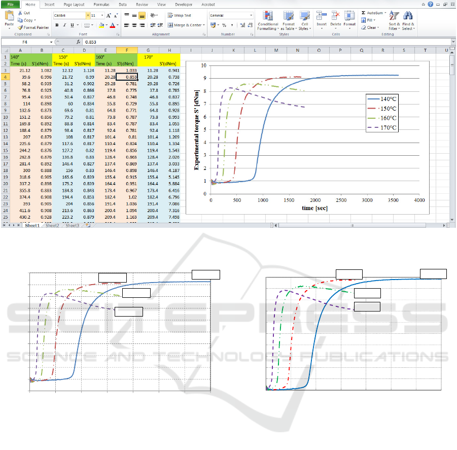
Figure 1: Excel file used to load experimental rheometer curves (on the right the experimental curves obtained at four
different temperatures).
Figure 2: Experimental rheometer curves at temperatures from 130 to 170°C (left) and calculated vulcanization degree
curves from Sun and Isayev (2009) relationship (note: induction, i.e. the curve before scorch point, is not excluded from
computations).
experimental data are stored, with the range of
variability to search the scorch point, at each curing
temperatures. Times are typically expressed in
minutes.
Experimental data are stored into a standard
Excel file, which is classically constituted by two
columns per experimented temperature, as illustrated
in Figure 1, the first for the time and the second for
the measured torque.
To test GURU, a benchmark of practical interest
is considered relying into the isothermal curing of a
natural rubber blend with properties reported in
Table I. Data are at disposal from (Leroy et al.,
2013) and (Milani et al.; 2013). The blend has been
experimentally tested at five different temperatures,
from 130 to 170°C, with a temperature step equal to
10°C. Curve at 130°C reported by (Leroy et al.;
2013) and (Milani et al.; 2013) is not loaded into
GURU, because reversion is absent (as at 140°) and
the behaviour is very similar to that found at 140°C.
Optimization obtained in GURU at 130°C will be in
any case shown at the end of the paper, in order to
compare the kinetic constants so obtained with those
predicted with alternative approaches. A Moving
Die Rheometer MDR in dynamic mode (1 Hz) was
used to collect the experimental curves.
0
1
2
3
4
5
6
7
8
9
10
0 500 1000 1500 2000 2500 3000 3500
Experimental torque S' [dNm]
time [sec]
170°C
160°C
150°C
140°C
0%
10%
20%
30%
40%
50%
60%
70%
80%
90%
100%
0 500 1000 1500 2000 2500 3000 3500
Vulcanization degree [%]
Time [sec]
170°C
160°C
150°C
140°C
Interactive GUI Software for Natural Rubber Vulcanization Degree Numerical Prediction
159
Figure 3: Explanation of the GUI software used to heuristically optimize the kinetic model on the available experimental
data.
Figure 4: GUI after graphical optimization on experimental data.
The torque
()
tS'
experimentally determined can
be then used to estimate the vulcanization degree
()
t
exp
α
, using the following relationship proposed
by (Sun and Isayev; 2009):
()
()
00
minmax
min
exp
'
TT
T
SS
StS
t
−
−
=
α
(1)
where
T
S
min
is the S’ minimum value at
temperature T. Before reaching this minimum value,
()
t
exp
α
is considered equal to zero. S
min T0
and S
max
T0
are the minimum and maximum torque values at a
curing temperature equal to T0 low enough to allow
neglecting reversion. In other words, the low
temperature “reversion free” increase of mechanical
properties during cure is taken as a reference, to
estimate the influence of reversion at higher
temperatures, which obviously results in a final
degree of vulcanization lower than 100%. In our
case the reversion free reference temperature is
0 20 40 60
0
2
4
6
8
10
140°C
Torque [dNm]
0 10 20 30 40 50
0
0.2
0.4
0.6
0.8
1
Vulcanization degree
α
[ ]
Experimental
Numeric al
0 10 20 30 40 50
0
0.1
0.2
Time t [min]
Abs. error e=|f
exp
-f
num
|
2.25 2.3 2.35 2.4 2.45
x 10
-3
-12
-10
-8
-6
-4
-2
1/T [1/K]
ln(K
i
) K
i
in 1/sec
K
1
K
2
K
3
K
1
linear regression
K
2
linear regression
K
3
linear regression
0 10 20 30
0
2
4
6
8
10
150°C
0 5 10 15 20 25
0
0.2
0.4
0.6
0.8
1
Experimental
Numeric al
0 5 10 15 20 25
0
0.1
0.2
Time t [min]
0 10 20 30
0
2
4
6
8
160°C
0 10 20 30
0
0.2
0.4
0.6
0.8
1
Experimental
Numerical
0 10 20 30
0
0.1
0.2
Time t [min]
0 10 20 30
0
2
4
6
8
170°C
0 10 20 30
0
0.2
0.4
0.6
0.8
1
Experimental
Numeric al
0 10 20 30
0
0.1
0.2
Time t [min]
SIMULTECH 2016 - 6th International Conference on Simulation and Modeling Methodologies, Technologies and Applications
160

either 140 or 130°C, providing both temperatures
very similar results.
Normalization Equation (1) is implemented into
GURU and allows to pass from experimented torque
to normalized torque, used to interactively fit
numerical data.
Figure 2 shows the typical torque- curing time
curves obtained experimentally at the different
vulcanization temperatures. As can be noted, the
reversion phenomenon, which can be clearly
observed at 160 and 170°C, almost vanishes at
140°C, where the torque clearly reaches a horizontal
plateau at the end of the experiments. A very similar
rheometer curve is obtained at 130°C.
3 THE KINETIC MODEL BY HAN
The basic reaction schemes used in the software are
classic, and basically refer to the so-called Han’s
model (Han et al., 1998).
As universally accepted, many reactions occur in
series and parallel during NR cured with sulphur.
After a viscous phase which characterizes the
uncured rubber at high temperature and called
“induction”, the chain reactions are initiated by the
formation of precursors, characterized by the kinetic
constant
1
K
.
Table 1: Rubber blend composition tested in rheometer
experimentation.
Component
Parts (by weight)
Rubber gum 100
Carbon black 25
Oil 5
(ZnO / Stearic acid) 6
Sulphur 3
amine antioxidant 2
Then, curing proceeds through two pathways,
with the formation of stable and unstable unmatured
cured rubber. The distinction between stable and
unstable curing stands in the presence of single or
multiple sulphur bonds respectively. Multiple S-S
bonds are intuitively less stable, and the evolution to
matured cross-linked rubber is again distinct
between the single S link between chains and the
multiple one, statistically much less stable and
leading to break and backbiting with higher
probability.
All the reactions considered occur with a kinetic
velocity depending on the curing temperature,
associated to each kinetic constant.
Let us assume that
i
K
is the i-th kinetic
constant associated to one of the previously
described phases, so that
0
K
describes induction,
1
K
and
2
K
the formation of unmatured polymer,
one stable and the other unstable, and
3
K
describes
reversion.
Within such assumptions, we adopt for NR the
kinetic scheme constituted by the chemical reactions
summarized in the following set of equations:
[][]
[]
*
1
0
ASA
k
c
→+
[][]
*
1
*
1
1
RA
k
→
[]
[]
1
*
1
2
RA
k
→
[]
[]
D
k
RR
11
3
→
(2)
In Equation (2),
[]
c
A
is a generic accelerator,
[]
S
is sulphur concentration,
[
]
*
1
A
the sulphurating
agent,
[
]
*
1
R
the stable crosslinked chain (S-S single
bonds),
[]
1
R
the unstable vulcanized polymer,
[
]
D
R
1
the de-vulcanized polymer fraction
(reversion).
3,2,1,0
K
are kinetic reaction constants.
Here it is worth emphasizing that
3,2,1,0
K
are
temperature dependent quantities, hence they
rigorously should be indicated as
()
TK
3,2,1,0
, where
T
is the absolute temperature. In what follows, for
the sake of simplicity, the temperature dependence
will be left out.
The interaction between
1
K
and
2
K
, from a
chemical point of view, is associated with the
formation of the activated complex and hence is
linked to the activity and concentration of
[
]
*
1
A
.
3
K
is reported by Han 0 to be responsible for
reversion after the peak torque, as chemically
confirmed by reactions in (2).
Interactive GUI Software for Natural Rubber Vulcanization Degree Numerical Prediction
161
150°C
160°C 170°C
Figure 5: Numerical and experimental normalized
rheometer curves. Comparison among GURU, Milani and
Milani (2015) and Leroy et al. (2013) approaches.
0
K
is the kinetic constant representing the
induction period, that can be excluded from the
computations assuming that the induction is
evaluated by means of a first order Arrhenius
equation.
According to the reaction scheme (2), excluding
induction, the following differential equations may
be written:
[
]
()
[]
*
121
*
1
AKK
dt
Ad
+−=
[
]
[]
*
11
*
1
AK
dt
Rd
=
[]
[]
[]
13
*
12
1
RKAK
dt
Rd
−=
(3)
The first Equation (3) may be trivially solved by
separation of variables, as follows:
[
]
[
]
()()
i
ttKK
eAA
−+−
=
21
0
*
1
*
1
[
]
[]
()()
i
ttKK
eAK
dt
Rd
−+−
=
21
0
*
11
*
1
[]
[]
()()
[]
13
0
*
12
1
21
RKeAk
dt
Rd
i
ttKK
−=
−+−
(4)
Once
[
]
*
1
A
is a known analytical function,
[
]
*
1
A
can be substituted into equations (b) and (c) in
(4) to provide
[
]
*
1
R
and
[]
1
R
:
[]
[
]
()()
[]
i
ttKK
e
KK
AK
R
−+−
−
+
=
21
1
21
0
*
11
*
1
[]
[]
[]
()()
i
ttKK
eAKRK
dt
Rd
−+−
=+
21
0
*
1213
1
(5)
The second Equation (5) is a non homogeneous
first order linear differential equation, which admits
the following solution constituted by a general and a
particular root:
[]
[]
() ( )()
[]
izi
ttKKttK
eeA
KKK
K
R
−+−−−
−
−+
=
=
13
0
*
1
321
2
1
(6)
The final concentration of vulcanized rubber is
thus
[
]
*
1
R
+
[]
1
R
:
[]
[]
[
]
()()
[]
[]
() ( )()
[]
ii
i
ttKKttK
ttKK
eeA
KKK
K
e
KK
AK
RR
−+−−−
−+−
−
−+
+
+−
+
=+
213
21
0
*
1
321
2
21
0
*
11
*
11
1
(7)
(7) can be normalized with respect to
[]
0
S
as
follows to provide the crosslinking density
α
:
[]
[
]
[]
()()
[]
() ( )()
[]
ii
i
ttKKttK
ttKK
ee
KKK
K
e
KK
K
S
RR
−+−−−
−+−
−
−+
+
+−
+
=
+
=
213
21
321
2
21
1
0
*
11
1
α
(8)
4 SOFTWARE ENGINE
GURU core appears to the user immediately after
having stored the experimental Excel database, as in
Figure 1.
With reference to Figure 3, where GURU
interface is shown before any optimization, the
software is roughly organized into five columns.
0 5 10 15 20 25
0
0.1
0.2
0.3
0.4
0.5
0.6
0.7
0.8
0.9
1
time [min]
α
crosslink density or normalized torque
GURU
Milani & Milani (2015)
Leroy et al. (2013)
Experimental data
0 5 10 15 20 25 30
0
0.1
0.2
0.3
0.4
0.5
0.6
0.7
0.8
0.9
1
time [min]
α
crosslink density or normalized torque
GURU
Milani & Milani (2015)
Leroy et al. (2013)
Experimental data
0 5 10 15 20 25 30
0
0.1
0.2
0.3
0.4
0.5
0.6
0.7
0.8
0.9
1
time [min]
α
crosslink density or normalized torque
GURU
Milani & Milani (2015)
Leroy et al. (2013)
Experimental data
SIMULTECH 2016 - 6th International Conference on Simulation and Modeling Methodologies, Technologies and Applications
162

The first four columns from the left represent
synoptically data at a given vulcanization
temperature, starting for instance from 140°C with
the column on the left and ending with 170° in the
fourth column on the right (see detail A in Figure 3).
Each column represents on the top the crude
experimental rheometer data (detail B), with an
indication of the scorch time adopted (yellow dot
moving on the curve after user’s action 1 on the top
slider in Figure 3), the performance of the numerical
model (detail D) with respect to normalized
experimental curve (detail C) in the central sub-
figure and the absolute error of the numerical model
when compared with normalized experimental curve
(detail E).
Kinetic constants are dynamically modified by
means of user’s action on the sliders on the bottom
(action 2). A user can dynamically move the slider
by means of a trial and error procedure in order to
graphically minimize the absolute difference
between experimental and numerical curve. Scorch
point can be adjusted as well. Typically, the
optimization of the parameters takes few instants.
The values of the kinetic constants are dynamically
updated and registered in the table situated on the
bottom left part of the screen (detail 4) and plotted in
the Arrhenius space depicted on the top-left (detail
3). In the same sub-figure, the linear regression of
each kinetic constant is also represented.
An indication of the stored Excel file name is
also provided in a yellow box (detail F).
Finally, data obtained after proper trial and error
interactive optimization can be saved by means of a
standard “Save” button located on the top-right
region of the interface. After having pressed the
button, a standard saving interface appears. By
default, it is possible to save data in a desired folder
with any output name in “.dat” format, which is the
standard binary format for Matlab. Files with
extension “.dat” are immediately available at any
time by any user, after proper reloading in a new
Matlab session. By default GURU loads at the
beginning a file called “output_data.dat”. In this
way, after a first optimization session, the user can
modify in successive sessions the work previously
saved and properly reloaded.
5 AN EXAMPLE OF TECHNICAL
RELEVANCE
GURU reliability is tested on some existing
experimental data from (Milani et al., 2013) and
Leroy et al. (2013). Attention is focused exclusively
on the fitting capabilities. GURU interface, after a
quick trial and error optimization session is shown in
Figure 4. As can be noted from the details of the
fitting quality at each temperature and the estimated
kinetic constants in the Arrhenius space, both good
agreement with normalized experimental data and
almost perfect linearity of the kinetic constants is
experienced.
Since output data obtained may be saved in a
proper database (file .dat into Matlab environment,
with kinetic constant values directly at disposal in
the command window for additional computations)
with the dedicated “save” button on the top-right of
GURU (see Figure 3), a more detailed insight into
the fitting quality obtained with the graphical
procedure can be also provided.
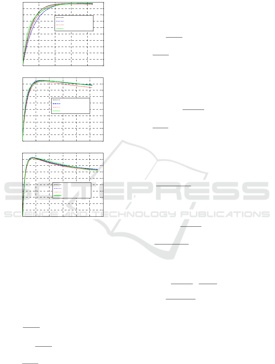
In particular, normalized rheometer curves
obtained by means of GURU are depicted in Figure
5 and compared with normalized experimental data
and numerical curves obtained in (Leroy et al.,
2013) and (Milani and Milani, 2015) with a least
square and interactive simplified semi-analytical
approach, respectively.
GURU fits well experimental results, sometimes
better than expensive least-squares approaches.
Figure 6: GURU performance in the Arrhenius space for
the determination of Ki constants at different temperatures
in the Arrhenius space. Comparison with other approaches
presented in the technical literature.
The numerical rheometer curve is very near to
the experimental one in absence of reversion, i.e. at
low temperature (140°C), but appears extremely
satisfactory even in presence of visible reversion
(170°C). The absolute error appears constantly lower
than 0.1 (i.e. with a relative error normalized on the
unitary maximum torque equal to 10%) in case of
both strong and zero reversion, a result which
appears fully acceptable for practical purposes. From
simulations results, it is interactively found that the
kinetic constants follow reasonably well linearity in
2.2 2.25 2.3 2.35 2.4 2.45 2.5 2.55 2.6
x 10
-3
-13
-12
-11
-10
-9
-8
-7
-6
-5
-4
-3
1/T [K
-1
]
ln(K
i
) [K
i
in 1/sec]
K
1
GURU
K
1
GURU linear regression
K
1
Milani & Milani (2015)
K
1
Milani & Milani (2015) linear regression
K
1
Leroy et al. (2013)
K
1
Leroy et al. (2013) linear regression
K
2
GURU
K
2
GURU linear regression
K
2
Milani & Milani (2015)
K
2
Milani & Milani (2015) linear regression
K
2
Leroy et al. (2013)
K
2
Leroy et al. (2013) linear regression
K
3
GURU
K
3
GURU linear regression
K
3
Milani & Milani (2015)
K
3
Milani & Milani (2015) linear regression
K
3
Leroy et al. (2013)
K
3
Leroy et al. (2013) linear regression
Interactive GUI Software for Natural Rubber Vulcanization Degree Numerical Prediction
163

the Arrhenius space, see Figure 4 and a more
detailed representation in Figure 6 also with data at
130°C. Ki numerical results found by (Leroy et al.,
2013) and (Milani and Milani, 2015), with the
corresponding linear regressions are also represented
for comparison purposes. The agreement between
GURU and (Leroy et al., 2013) is almost perfect,
even with a more satisfactory linearity in GURU.
When dealing with (Milani and Milani, 2015), the
agreement is rather good for K
1
and K
3
, but with
visible deviation at lower temperatures (130°C and
140°C) for K
2
, mainly related to an intrinsic
limitation of the semi-analytical approach proposed
in (Milani and Milani, 2015) (and hence independent
from GURU software).
From simulations results, it is interactively found
that the kinetic constants follow reasonably well
linearity in the Arrhenius space, see Figure 4 and a
more detailed representation in Figure 6 also with
data at 130°C. Arrhenius law represents one of the
most useful relationships in chemical kinetics, when
an extrapolation of the behavior is needed outside
the experimentally tested temperature range. In
Figure 6, we represent also Ki numerical results
found by (Leroy et al., 2013) and (Milani and
Milani, 2015), with the corresponding linear
regressions. Once again, we stress that (Leroy et al.,
2013) use Han’s model to fit experimental data and
Ki are evaluated by standard least-squares. (Milani
and Milani, 2015) again base on Han’s kinetic
scheme, but they propose, after few mathematical
considerations on the closed-form solution found to
estimate the crosslinking density, a semi-analytical
approach to estimate Kis, thus circumventing the use
of least-squares. As can be noted, the agreement
between GURU and (Leroy et al., 2013) approach is
almost perfect for all the kinetic constants, even with
a more satisfactory linearity experienced for GURU.
When dealing with (Milani and Milani, 2015)
procedure, the agreement with GURU appears again
rather good for K
1
and K
3
constants, but with visible
deviation at lower temperatures (130°C and 140°C)
for K
2
. Such inaccuracy is not surprising, and mainly
related to an intrinsic limitation of the semi-
analytical approach proposed by (Milani and Milani,
2015) and hence independent from GURU software.
As a matter of fact (Milani and Milani, 2015) closed
form solution requires an evaluation of K
2
through
the definition of the reversion percentage. When
reversion is absent or very small, K
2
is clearly
affected by high scatter. This also justifies the very
good agreement at 170 and 160°C, where reversion
is present.
REFERENCES
Colin X, Audouin L, Verdu J. Polymer Degradation and
Stability 2007; 92(5): 906–914.
Coran AY. Science and Technology of Rubber 1978,
Academic Press: New York, Chapter 7.
Ding R, Leonov I, Coran, AY. Rubber Chem Technol
1996; 69: 81.
Ding R, Leonov I. J Appl Polym Sci 1996; 61: 455.
Han IS, Chung CB, Kang SJ, Kim SJ, Chung HC. Polymer
(Korea) 1998; 22: 223-230.
Kamal MR, Sourour S. Polymer Engineering and Science
1973; 13: 59-64.
Leroy E, Souid, Deterre R.Polym. Test. 2013 ; 32: 575-
582.
Milani G, Hanel T, Milani F, Donetti R. Journal of
Mathematical Chemistry 2015; 53(4): 975-997.
Milani G, Leroy E, Milani F, Deterre R. Polymer Testing
2013; 32: 1052-1063.
Milani G, Milani F. Journal of Applied Polymer Science
2011; 119: 419-437.
Milani G, Milani F. Journal of Applied Polymer Science
2012; 124(1): 311–324.
Milani G, Milani F. Journal of Mathematical Chemistry
2015; 53(6): 1363-1379.
Milani G, Milani F. Polym. Test. 2014; 33: 1-15.
Milani G., Milani F. Journal of Mathematical Chemistry
2010; 48: 530–557.
Poh BT, Chen MF, Ding BS. Journal of Applied Polymer
Science 1996; 60: 1569-1574.
Poh BT, Ismail H, Tan ES. Polymer Testing 2002; 21:
801-806.
Poh BT, Tan EK. Journal of Applied Polymer Science
2001; 82: 1352-1357.
Sun X, Isayev AI. Rubber Chemistry and Technology
2009; 82(2):149-169.
Tanaka Y. Rubber Chemistry and Technology 1991; 64:
325.
SIMULTECH 2016 - 6th International Conference on Simulation and Modeling Methodologies, Technologies and Applications
164
