
Self-Diagnosing Low Coverage and High Interference in 3G/4G Radio
Access Networks based on Automatic RF Measurement Extraction
M. Sousa
2,3
, A. Martins
1,3
and P. Vieira
1,2
1
Instituto de Telecomunicac¸
˜
oes (IT), Lisbon, Portugal
2
Instituto Superior de Engenharia de Lisboa (ISEL), ADEETC, Lisbon, Portugal
3
CELFINET, Consultoria em Telecomunicac¸
˜
oes Lda., Lisbon, Portugal
Keywords:
Wireless Communications, SON, Self-Diagnosis, Coverage Detection, Interference Control.
Abstract:
This paper presents a new approach for automatic detection of low coverage and high interference scenarios
(overshooting and pilot pollution) in Universal Mobile Telecommunications System (UMTS) /Long Term Evo-
lution (LTE) networks. These algorithms, based on periodically extracted Drive Test (DT) measurements (or
network trace information), identify the problematic cluster locations and compute harshness metrics, at clus-
ter and cell level, quantifying the extent of the problem. Future work is in motion by adding self-optimization
capabilities to the algorithms, which will automatically suggest physical and parameter optimization actions,
based on the already developed harshness metrics. The proposed algorithms were validated for a live network
urban scenario. 830 3
rd
Generation (3G) cells were self-diagnosed and performance metrics were computed.
The most negative detected behaviors regards high interference control and not coverage verification.
1 INTRODUCTION
The increasing network complexity, in terms of num-
ber of monitored parameters and parallel operation of
2
nd
Generation (2G), 3G and 4
th
Generation (4G), is
increasing dramatically, besides the ever growing traf-
fic volume and service diversity. In the third quar-
ter of 2015, an average monthly data traffic of 4,700
petaBytes was registered, with an increase of 65%
compared with the third quarter of 2014 (Ericsson,
2015). This increases the network Operating Expense
(OpEx), forcing mobile operators to pursue strategies
for reducing it. Self-Organizing Networks (SON) al-
gorithms have been seen as the solution, and a way to
automatically operate the current and beyond mobile
networks.
This paper focus on the automatic-diagnosing al-
gorithms of low coverage and high interference sce-
narios, used to trigger optimization processes in self-
optimizing functions (within SON). Problem detec-
tion is based on periodically extracted DT measure-
ments or geo-positioned network traces (Vieira et al.,
2014). The DT data provides measurements of re-
ceived signal strength and quality for the different pi-
lot or reference signals that reach a certain location.
Moreover, specific filtering is applied to identify the
data that denotes either, coverage issues or interfer-
ence problems, such as overshooting or pilot pollu-
tion.
SON and self-diagnosing is a hot research topic
and recent work has been done leading to the cur-
rent research stage (Duarte et al., 2015),(Sousa et al.,
2015), (Sallent et al., 2011). The paper contribu-
tion is incremental to previous works. Firstly, the
used cell’s service area approximation based on prop-
agation modelling is more accurate when compared
with existent research. Secondly, a new cluster par-
tition approach using the auto-correlation distances
for shadow fading (Kysti et al., 2007), to limit clus-
ter size, results in a more coherent data analysis. Fi-
nally, this work address the DT minimization target of
3
rd
Generation Partnership Project (3GPP) by allow-
ing trace based inputs.
The aim of the present work is to be the cor-
nerstone in a fully self-optimization algorithm. This
work corresponds to the network data analysis phase,
which will report the detected areas with low perfor-
mance issues and all relevant data for the further opti-
mization algorithm. Additionally, harshness metrics
are already computed, accessing the cell’s detected
problems.
This paper is organized as follows. Section 2 de-
fines the scope embedding the present work. In sec-
tion 3 the concept of DT reliability is presented. Sec-
Sousa, M., Martins, A. and Vieira, P.
Self-Diagnosing Low Coverage and High Interference in 3G/4G Radio Access Networks based on Automatic RF Measurement Extraction.
DOI: 10.5220/0005958300310039
In Proceedings of the 13th International Joint Conference on e-Business and Telecommunications (ICETE 2016) - Volume 6: WINSYS, pages 31-39
ISBN: 978-989-758-196-0
Copyright
c
2016 by SCITEPRESS – Science and Technology Publications, Lda. All rights reserved
31
tion 4 presents the detailed self-diagnosing process
for each algorithm. The results are shown in section 5
and finally, in section 6, conclusions are drawn.
2 SELF-OPTIMIZATION
Self-Optimization, aims to maintain network quality
and performance with a minimum of manual inter-
vention. It monitors and analyses, either Key Per-
formance Indicator (KPI)s, DT measurements, traces
or other sources of information, triggering automated
actions in the considered network elements. The
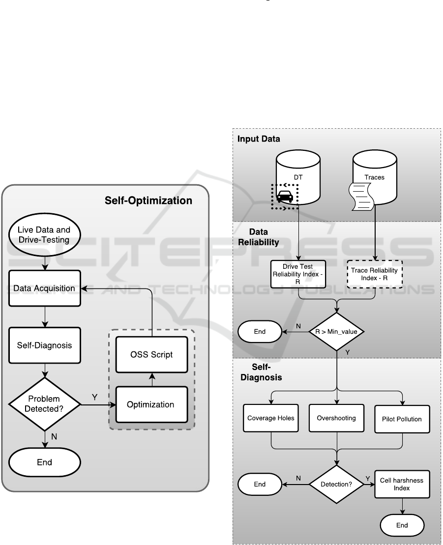
self-optimization process for a network under perfor-
mance enhancement is shown in Figure 1. This work
researches the Self-Diagnosis process block, hence
future work will complete the self-optimization func-
tion by implementing the optimization and Opera-
tional Support System (OSS) script blocks.
Figure 1: Global self-optimization flowchart.
The self-diagnosis module uses either DT mea-
surements or trace data as in Figure 2. Thus, with an
introduction of a reliability index R for the input data,
it accomplishes not only a control mechanism for the
self-optimization process, but also increases quality
in the self-diagnosis output. Only when the available
data, is significant to access the cell’s performance,
reflected by a value of R higher than a certain thresh-
old, min value, the self-diagnosis is executed. Oth-
erwise, the available information is not sufficient to
retain any strong conclusion. Furthermore, regarding
the trace reliability block, it is under development.
The self-diagnosis module is composed by three
different algorithms, coverage holes, overshooting
and pilot pollution, see Figure 2. For all of them, the
concerning data in the network optimization scenarios
is grouped in clusters. Moreover, a harshness index
H
cell
is calculated accessing the problem’s severity in
the cell.
Figure 2: Self-diagnosis flowchart.
WINSYS 2016 - International Conference on Wireless Networks and Mobile Systems
32

3 DRIVE-TEST DATA
CLASSIFICATION
There is an undeniable correlation in the assertiveness
of the DT based algorithm results and the complete-
ness of a DT campaign. As well, the harshness met-
rics will be as accurate as the DT is complete or sig-
nificant. This highlights the importance of a quality
metric associated with the DT used in any algorithm.
Hence, an assessment of the DT quality is executed
before the use of DT data itself, giving origin to a DT
reliability index R (Sousa et al., 2015). It evaluates the
data collected in a cell’s service area, taking into ac-
count the percentage of measurements collected and
its spatial distribution.
3.1 DT Spatial Distribution
The quadrant method is a statistical spatial analysis
method used as a mean to test a population point pat-
tern (random, clustered and dispersed). In this con-
text, the method is not used to classify the DT mea-
surements on its geographical distribution pattern, but
as a relative measurement of the dispersion level. This
allows to quantify how well distributed are the DT
measurements in the cell’s service area.
For that purpose, the service area is divided into
quadrants and the number of DT measurements on
each accounted. Figure 3 shows a cell’s service area
divided into equal areas, before applying the method.
Figure 3: Cell’s geographical area.
Considering the quadrant method data,
[Y (A
m
)]
P
= [x
1
, ..., x
m
] (1)
where x
m
is the number of measurements in the m
quadrant, for all A
m
quadrants covering the service
area P. Using this data set, a parameter that quantifies
the DT data pattern is calculated.
The parameter Variance to Mean Ratio (VMR)
allows to identify the distribution pattern of a data set
and it is given by,
V RM =
s
2
¯x
(2)
where s
2
is the variance of the number of measure-
ments and ¯x the average measurement number in each
quadrant. When the VMR value is higher than one,
the pattern is clustered. Below the unit is dispersed
and if it’s equal to one, the pattern is random. Due
to the direct correlation between DT measurements
and the own existence of roads, the pattern can’t be
random and hardly will ever be dispersed. So, the rel-
evant information is how much clustered might be.
This knowledge is reflected in the Dispersion In-
dex D
i
for a cell i. Using Equation (2) over the data
set given by Equation (1) the DT data dispersion in
the cell’s service area is calculated (V RM). The Dis-
persion Index D
i
, results from the normalization of
the DT data V MR, given by,
D
i
= 1 −
V RM
V RM
max
(3)
where V RM
max
is calculated using Equation 2 in the
case of all measurements being in one single area A,
thus resulting in a relative value of the data distribu-
tion.
3.2 Road Filling Ratio for DT
Measurements
The aim is to calculate the road filling ratio, P
i
, which
represents the percentage of road/street covered in the
service area of cell i. In order to proceed, the road net-
work information is fetched using an Application Pro-
gramming Interface (API). The obtained points are
linearly interpolated, for resolution purposes, result-
ing as shown in Figure 4.
An important piece of information, is the treat-
ment that the original geospatial positioned measure-
ments, enroll. They are subsequently aggregated on
geographical areas of ten by ten meters, called bins.
This term refers to several measurements from dif-
ferent cells aggregated in the same area, and will be
mentioned throughout this paper. To refer to a sin-
gle cell measurement contained in a bin, we refer as
a cell sample. Bearing in mind this information, the
same procedure must be applied to the retrieved road
points. Only then P
i
is calculates as,
P
i
=
M
Max
m
(4)
Self-Diagnosing Low Coverage and High Interference in 3G/4G Radio Access Networks based on Automatic RF Measurement Extraction
33
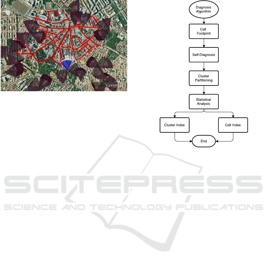
Figure 4: Street data information.
where M is the number of collected bins and Max
m
the equivalent of bins for all the road/street extension
in the service area of a cell i.
3.3 Calculating the DT Reliability Index
The DT Reliability Index R
i
, gets values in the zero to
one range, and it merges the previous two metrics, in
the following way,
R
i
= α
d
D
i
+ α
p
P
i
(5)
where α
d
is the weight of the dispersion index D
i
,
for cell i and α
p
is the weight of the percentage of
road covered P
i
, in cell i. Regarding the weights of
both factors (α
d
and α
p
) they resulted from empirical
knowledge, through a statistical analyze of fifty DT
classification inquiries, performed to Celfinet’s expe-
rienced radio engineers (Sousa et al., 2015).
4 THE SELF-DIAGNOSIS
PROCESS
The underlying process for the identification of either
coverage holes, overshooting or pilot pollution sce-
narios has a common ground. The goal is always, re-
garding the specific algorithm, to diagnose prevalent
under performance situations in the form of clusters.
Furthermore, to attribute a harshness metric based on
a statistical analysis to each cluster, and a harshness
level of the cell, due to all clusters found, as presented
in Figure 5.
4.1 Self-Diagnosis Modules
As stated before, in this work three detection algo-
rithms are presented. This subsection characterizes
Figure 5: General detection flowchart.
each algorithm, in terms of the data identification pro-
cess.
4.1.1 Detecting Coverage Holes
A coverage hole is defined as an area where the pi-
lot (or reference) signal power is in between the low-
est network access threshold and the lowest value re-
quired for assigning full coverage. Users in this area
tend to suffer poor voice or data user experience and
possibly dropped calls or high latency.
From the cell’s footprint, a coverage hole sample
must accomplish two conditions. Firstly, it must be
best server or within a small power interval to the best
server of the respective bin. To these, we will refer
as serving samples. Note that best server is the mea-
surement that corresponds to the best cell, and that
should serve the mobiles at that point. Secondly, the
best server measurement from the respective serving
sample bin, must be below the coverage threshold,
BS
power
< T hr
CH
(6)
where BS
power
is the best server value and T hr
CH
is
the minimum serving power value, which is tecnhol-
ogy (3G 4G) and use case dependent.
4.1.2 Detecting Overshooting
An overshooting situation occurs when the cell’s cov-
erage reaches beyond what is planned. Generally, oc-
WINSYS 2016 - International Conference on Wireless Networks and Mobile Systems
34

curs as an “island” of coverage in another cell’s ser-
vice area. Overshooted areas may also suffer from
call drops and bad quality of experience.
From the cell’s DT measurements, the ones con-
sidered in overshooting, must be located beyond the
cell’s service area. Then, to be considered overshoot-
ing, it must comply with the following conditions, re-
garding the power value measured,
(
CS
pwr
> T hr
OS
, if CS is best
CS
pwr
> Best
pwr
− ∆
pwr
, if CS is not best
(7)
where CS
pwr
is the cell sample power value, T hr
OS
is the minimum power value to be considered over-
shooting, Best
pwr
is the power value of the bin best
server cell and ∆
pwr
is used to define a power range to
consider overshooting. Two conditions are presented,
for the case when the corresponding sample of the cell
in analysis is the best server cell and for the opposite
case.
Also, the quality of the cell’s measurements is
evaluated, using the same conditions as Equation 7
but regarding the quality measurments,
(
CS
qual
> QT hr
OS
, if CS is best
CS
qual
> Best
qual
− ∆
qual
, if CS is not best
(8)
Not all overshooting situations are necessarily
damaging to the network or non-intended. Even
though effectively being far from the normal service
area, it might happen that, due to terrain profile, it
still might be the cell in best condition to serve in
that area. In that sense, in case of the majority of the
overshooting bins, containing the best server as the
analyzed cell and a delta value of power and quality
to the second best server, these will also be marked.
They will still be identified as overshooters and con-
tinue the process, but containing an observation that
optimizing this overshooting area might reduce the
overall network performance.
4.1.3 Detecting Pilot Pollution
Pilot pollution remarks a scenario where too many pi-
lots (or reference signals in the case of LTE) are re-
ceived in one area. Besides the excess of pilots, it
lacks a dominant one. These areas are highly inter-
fered, resulting in a poorer user experience.
The cell’s measurements inducing pilot pol-
lution, are in a serving ranking bellow the
ideal maximum number of cells serving in that
area. To the cell’s footprint where the previ-
ous is verified, the following conditions, must
be complied to be in a pilot pollution situation,
(
CS
pwr
> Best
pwr
− ∆
pwr
CS
qual
> Best
qual
− ∆
qual
(9)
where CS
pwr
is the cell sample power value, Best
pwr
is the power value of the bin best server cell and ∆
pwr
is used to define a pilot pollution power range. The
second condition is equal to the first, but regarding
quality measurements.
4.2 Cluster Partitioning
The radio mobile channel is uncertain due mainly to
the effects of fading and multipath. So, the values
caught on DT measurements, which are reported at
one single instance of time, may not correspond to
the average behavior of the radio channel in that point.
In order to mitigate this variability, the detection pro-
cess is executed at the cluster level and not at bin
level. This enables to detect prevailing under perfor-
mance areas and not simply variations, normal and
non-correlated with network issues. Therefore, us-
ing the auto-correlation distances for shadow fading
(Kysti et al., 2007), to limit cluster size, this gives
more assertiveness in the detected results.
Regarding the cluster division process itself, it
is accomplished using a dendrogram structure (Izen-
man, 2008). It is a tree diagram that, in this applica-
tion, translates the distance relation between all DT
measurements detected, as can be seen in Figure 6.
The tree diagram building process, aggregates succes-
Figure 6: Dendrogram tree structure.
sively the closest bin/cluster pair until all of the bins
form a unique cluster. At each aggregation, is con-
structed a different cluster division possibility.
The next step is to define which cluster arrange-
ment is best. Several algorithms accomplish this pur-
pose, and throw different metrics and approaches. But
overall what they evaluate is how well concentrated
are the points in clusters, when the distance similarity
(Zheng and Xue, 2009) is high. The approach used
was the silhouette method (Witten and Frank, 2005).
It provides a metric s(i),
s
i
=
b(i) −a(i)
max{a(i), b(i)}
(10)
Self-Diagnosing Low Coverage and High Interference in 3G/4G Radio Access Networks based on Automatic RF Measurement Extraction
35

where a(i) is the average dissimilarity to the other
points of the cluster, b(i) the lowest average dissimi-
larity of i to any other cluster. It evaluates how well
any given point lies within its cluster. Thus, an s(i)
close to one means that the bin is appropriately clus-
tered. This approach is only applied to the cluster di-
vision possibilities that respect the maximum cluster
size due to the correlation distance.
4.3 Cluster Statistical Analysis
A statistical analysis is conducted to each detected
cluster. The purpose is to classify the harshness
(severity of the problem) and rank by it. The result
is a harshness index, H
cluster
, per cluster, given by,
H
cluster
=
∑
N
i=1
β
i
U(c(i))
∑
N
i=1
β
i
, 0 ≤ H
cluster
≤ 1 (11)
where β
i
is the weight for condition i and the U(c(i)),
U(c(i)) =
(
1, if c(i) is full field
0, otherwise
(12)
, are the evaluated conditions. Once again these con-
ditions are dependent on the behavior that is being
analyzed.
The coverage hole algorithm calculates it’s H
cluster
index (11) using the following conditions:
C(1) : Prob(Power
s
≤ Power
cov
) ≥ T hr
CH
(13)
C(2) : Prob(Power
n
≤ Power
cov1
) ≥ T hr
CH
(14)
where Power
s
is the cell’s power measurement
value, Power
cov
is a coverage threshold and T hr
CH
is the minimum percentage of data samples that are
below the coverage value, so that the condition is ful-
filled. The variable Power
n
is the power measurement
value of a neighbor cell, who also serves that area.
The Power
cov1
is just another power value to be com-
pared with. These conditions allow to classify the
harshness of a coverage hole in two forms. The con-
dition from Equation (13) concerns only to the power
value of the source cell. Using different Power
cov
val-
ues and different percentages T hr
Power
a cluster will
be classified more or less harsh. The second condi-
tion, in Equation (14), evaluates the existence of other
fallback cell in the cluster.
The coverage hole harshness index H
cell
repre-
sents a percentage of clusters in coverage hole versus
the clusters of the cell footprint.This metric might be
devious, especially if the DT data are low in number.
In that case, the metric will exceed the true percent-
age value. That’s why the DT reliability index R is so
important in terms of interpreting the results.
The overshooting cluster harshness evaluation
proceeds with the following conditions:
C(1) : Prob(Power
s
≥ Power
OS
) ≥ T hr
OS
(15)
C(2) : Prob(Power
s
≥ Power
OS1
) ≥ T hr
OS
(16)
C(3) : Prob(Qual
deg
≥ Qual
degOS
) ≥ T hr
OS
(17)
where Power
OS
and Power
OS1
are different power val-
ues to be compared with. The conditions from Equa-
tion (15) and Equation (16) are exactly the same,
but using different Power
OS
values, evaluating the
power level of the overshooting, allowing more res-
olution in distinguishing overshooting clusters in se-
vere terms. The condition from Equation 17, evalu-
ates the quality degradation caused by the existence of
an overshooting cell (Sanchez-Gonzalez et al., 2013),
in which Qual
deg
is the quality degradation caused
and Qual
degOS
is a quality degradation threshold.
The overshooting harshness index H
cell
repre-
sents the average percentage of overshooting clusters
against the victim cells footprint, divided also in clus-
ters. Once again, the importance of the DT reliability
index must be highlighted.
Concerning the pilot pollution algorithm, the con-
ditions to evaluate the harshness level are the follow-
ing:
C(1) : Prob(Power
best
≥ Power
PP
) ≥ T hr
PP
(18)
C(2) : Prob(Qual
deg
≥ Qual
degPP
) ≥ T hr
PP
(19)
where Power
best
is the signal power of the best server
measurement and Power
PP
is a threshold value to be
compared with. The condition presented in Equation
(18), reflects that, a pilot pollution scenario is as dam-
aging to the network as higher is the power of the
correspondent best servers. The second condition (in
Equation (19)), as seen in the overshooting, gauge the
quality degradation that the source cell induces on the
best servers.
In case of the pilot pollution algorithm, being a
scenario where cells affect another cell performance,
the approach for the pilot pollution harshness index
H
cell
is the same as described in the overshooting
module.
5 APPLYING THE ALGORITHM
TO A LIVE NETWORK
The developed algorithms were applied in a live net-
work, and for an urban scenario. 830 3G cells oper-
ating at different frequencies were self-diagnosed and
performance metrics were computed. Extensive DT
data corresponding to this area was used.
WINSYS 2016 - International Conference on Wireless Networks and Mobile Systems
36
5.1 Overview Details
Regarding to the thresholds used in section 4.1) to
identify the intended network behaviors, they are ex-
tremely dependent on mobile operator policies, re-
quirements, type of service, etc., so a set of default
parameters was used, as detailed in Table 1. The over-
all results are shown in Table 2. The columns ”CH”,
”OS” and ”PP” refer to coverage holes, overshooting
and pilot pollution algorithms, respectively.
Table 1: Algorithms thresholds and inputs.
CH OS PP
RSCP
threshold [dBm]
-100 -95 -95
RSCP
delta [dB]
3 6 6
Min EcN0
threshold [dB]
N/A -10 N/A
EcN0
delta [dB]
N/A 6 4
Number
of bins / cluster
10 10 10
Max
cluster radius [m]
57,5 57,5 57,5
Pilot
pollution window
N/A N/A 3
The results on Table 2, reveal a considerable num-
ber of cells with performance malfunctions, which are
currently under more detailed evaluation by radio op-
timization teams. In terms of the coverage hole index
H
cell
, it is the highest. The DT reliability index R is
Table 2: Self-diagnosis detected scenarios.
CH OS PP
Analyzed cells 830
Detected cells 13 35 64
Average clusters [#] 3 2 3
Average index H
cell
[%] 38 11 11
Average index R [%] 37 45 55
the lowest, though. Which admits that the DT did not
retrieve data from all cell service area, leading to an
overestimated H
cell
value. With regard to the interfer-
ence detection algorithms, the average cell index H
cell
was 11% with more quality of the respective DT data.
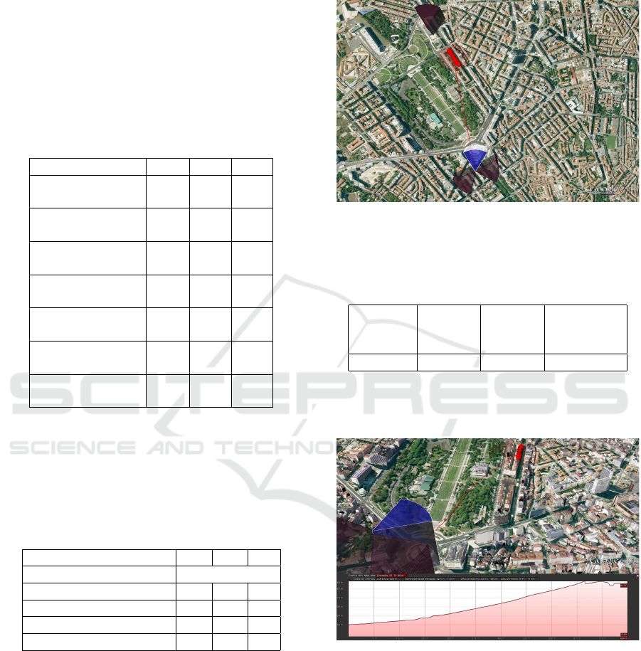
5.2 Coverage Holes
One of the detected coverage holes is illustrated in
Figure 7. The blue cell is the diagnosed cell, with the
red points corresponding to the cell’s measurements
in coverage hole, grouped in one cluster.
Figure 7: Coverage hole scenario.
The detailed Radio Frequency (RF) metrics are
displayed in Table 3. It can be observed the -103 dBm
Table 3: Coverage hole measurements details.
Number
of bins
Average
RSCP
[dBm]
Average
Ec/No [dB]
Cluster 1 14 -103 -9
low signal power level, on average, for the 14 detected
measurements.
Figure 8: Coverage hole cluster terrain profile.
Using software with elevation profiling and 3D
building modulation, see Figure 8, it can be asserted
that the coverage hole area is in Non-Line-of-Sight
(NLoS) due to building obstruction and terrain eleva-
tion.
In relation to the index H
cell
, for this occurrence,
it was 25%, meaning that 25% of the clusters are in
coverage hole. Nevertheless, as the DT reliability in-
dex R for the cell was only 23%, it may indicate that
the index S be off the real percentage.
Self-Diagnosing Low Coverage and High Interference in 3G/4G Radio Access Networks based on Automatic RF Measurement Extraction
37
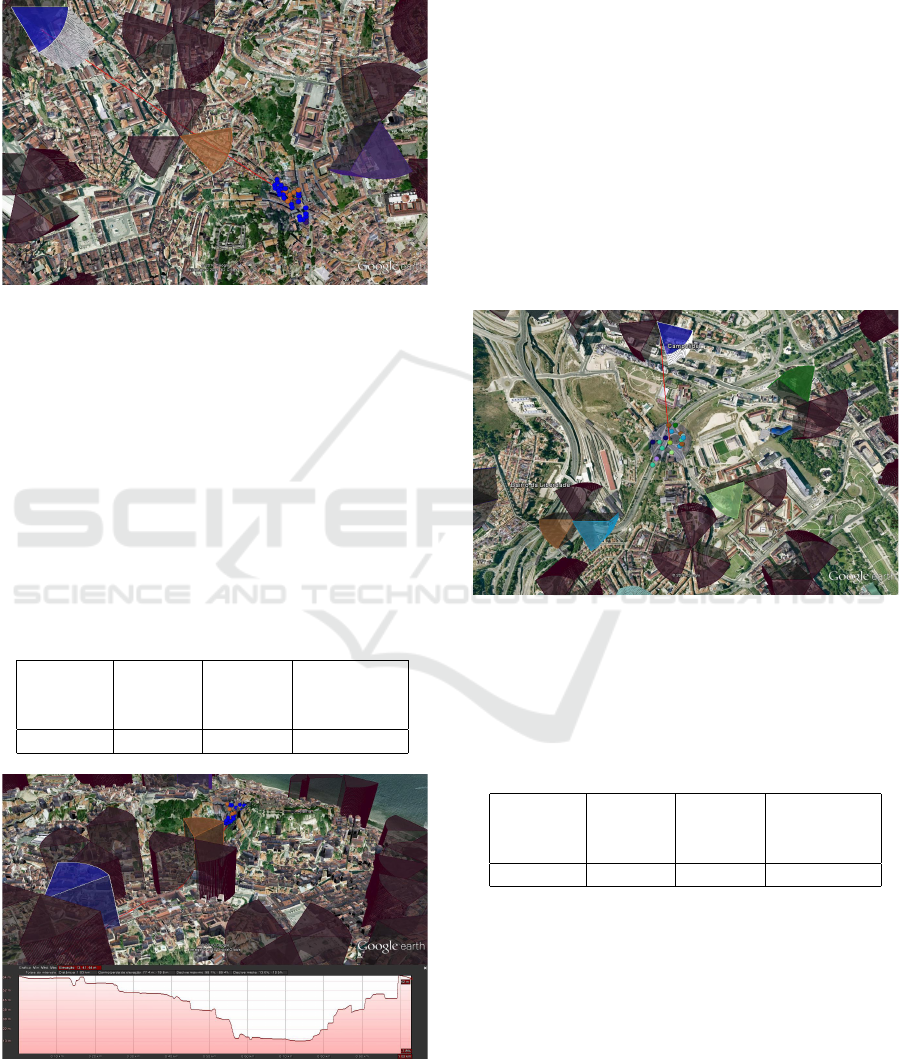
5.3 Overshooting
Concerning the overshooting, Figure 9, illustrates an
overshooting in an overlap area between two cells.
Figure 9: Overshooting scenario.
Again, the blue cell is the diagnosed cell, and in
this case, it was detected an overshooting cluster. Fur-
thermore, the cells with orange and purple, were iden-
tified as the victim cells, in the sense that, the over-
shooting cluster is located in their service areas. The
measurement stats are shown in Table 4. The blue cell
is reaching the other two cell service areas with a high
power, causing interference.
Just for additional information, see Figure 10,
where the terrain profile between the source cell and
the respective overshooting cluster is illustrated, con-
firming the ”high pass”.
Table 4: Overshooting measurements details.
Number
of bins
Average
RSCP
[dBm]
Average
Ec/No [dB]
Cluster 1 31 -69 -9
Figure 10: Overshooting cluster terrain profile.
It exists Line-of-Sight (LoS) between the source
cell and the overshooting cluster which enables the
overshooting scenario. In regard to the overshooting
cell index, H
cell
, it was obtained a value of 9%. This
represents, in this particular case, that the overshoot-
ing clusters affected, on average, 9% of the victim
cells footprint divided in clusters. Concerning the DT
reliability index R, it was obtained an average value
of 41% for the two victim cells.
5.4 Pilot Pollution
Regarding the pilot pollution detection algorithm, an
example is illustrated in Figure 11. The diagnosed
cell (in blue) is reaching an area, within the pilot pol-
lution conditions (4.1.3), where the red, green and
light purple cells are the serving (best) cells in that
area. The detected pilot pollution bins, were arranged
in one valid cluster.
Figure 11: Pilot pollution scenario.
The pilot pollution average metrics are presented
in Table 5. Even for the high average power detected,
the average quality level is very low, exhibiting how
interfered is this area.
Table 5: Pilot pollution measurements details.
Number
of bins
Average
RSCP
[dBm]
Average
Ec/No [dB]
Cluster 1 17 -77 -17
It can be seen in Figure 12 that the NLoS scenario
is not enough to reduce the source power received.
Due, mainly, to the relative small distance between
the cluster and the source cell, besides that, this cell
operates in the 900 MHz band.
In terms of the cell severity index H
cell
, for this
case the reported value, was 14%. It shows that the
pilot pollution clusters are in average 14% of the de-
tected serving cells footprint. In the matter of the DT
reliability index of the victim cells, was retrieved an
average value of 62%, which empowers greatly this
WINSYS 2016 - International Conference on Wireless Networks and Mobile Systems
38

Figure 12: Pilot pollution cluster terrain profile.
pilot pollution H
cell
index, compared to the overshoot-
ing harshness index.
By definition, pilot pollution areas display an ex-
cessive number of pilot signals. Sometimes, this num-
ber is high enough, that enables the algorithm to sug-
gest which cell(s) are being victimized. In this sce-
nario, the detection is done, but insufficient informa-
tion retains the algorithm from the harshness evalua-
tion and the affected cell identification.
6 CONCLUSIONS
This paper presented a new approach for automatic
detection of low coverage and high interference sce-
narios (overshooting and pilot pollution) in UMTS
/LTE networks. These algorithms, based on period-
ically extracted DT measurements, identify the prob-
lematic cluster locations and compute harshness met-
rics, at cluster and cell level, quantifying the extent of
the problem.
The proposed algorithms were validated for a live
network urban scenario. 830 3G cells were self-
diagnosed and performance metrics were computed.
The results showed that for an urban area and with
a high site density, the main optimization efforts rely
on the interference mitigation and not coverage opti-
mization. Moreover, the pilot pollution scenarios are
the most prevalent.
The cluster division, with a RF correlation dis-
tance limitation, provides a simplification for the an-
tenna physical parameter optimization algorithms, in
the sense that, the optimization process can be re-
duced to the cluster’s centroids.
Future work is in motion by adding self-
optimization capabilities to the algorithms, which will
automatically suggest physical and parameter opti-
mization actions, based on the already developed
harshness metrics.
ACKNOWLEDGEMENTS
This work was supported by the Instituto de
Telecomunicac¸
˜
oes (IT) and the Portuguese Founda-
tion for Science and Technology (FCT) under project
PEst-OE/EEI/LA0008/2013.
REFERENCES
Duarte, D., Vieira, P., Rodrigues, A. J., and Silva, N. (2015).
A new approach for crossed sector detection in live
mobile networks based on radio measurements. In
Wireless Personal Multimedia Communications Symp.
- WPMC, volume 1.
Ericsson (2015). Ericsson mobility report. Technical report,
ERiCSSON.
Izenman, A. J. (2008). Modern Multivariate Statistical
Techniques: Regression, Classification, and Manifold
Learning. Springer Publishing Company, Incorpo-
rated, 1 edition.
Kysti, P., Meinil, J., Hentil, L., Zhao, X., Jms, T., Schnei-
der, C., Narandzi, M., Milojevi, M., Hong, A., Ylitalo,
J., Holappa, V., Alatossava, M., Bultitude, R., Jong,
Y., and Rautiainen, T. (2007). Ist-4-027756 winner ii
d1.1.2 v1.2. Technical report, EBITG, TUI, UOULU,
CU/CRC, NOKIA.
Sallent, O., Perez-Romero, J., Sanchez-Gonzalez, J.,
Agusti, R., Diaz-Guerra, M., Henche, D., and Paul,
D. (2011). Automatic detection of sub-optimal perfor-
mance in umts networks based on drive-test measure-
ments. In Network and Service Management (CNSM),
2011 7th International Conference on, pages 1–4.
Sanchez-Gonzalez, J., Sallent, O., P
´
erez-Romero, J., and
Agust
´
ı, R. (2013). A multi-cell multi-objective self-
optimisation methodology based on genetic algo-
rithms for wireless cellular networks. Int. Journal of
Network Management, 23(4):287–307.
Sousa, M., Martins, A., Vieira, P., Oliveira, N., and Ro-
drigues, A. (2015). Caracterizacao da fiabilidade
de medidas r
´
adio em larga escala para redes auto-
otimizadas. In 9. Congresso do Comit
´
e Portugu
ˆ
es da
URSI - ”5G e a Internet do futuro”.
Vieira, P., Silva, N., Fernandes, N., Rodrigues, A. J.,
and Varela, L. (2014). Improving accuracy for otd
based 3G geolocation in real urban/suburban environ-
ments. In Wireless Personal Multimedia Communica-
tions Symp. - WPMC, volume 1.
Witten, I. H. and Frank, E. (2005). Data Mining: Practi-
cal Machine Learning Tools and Techniques, Second
Edition (Morgan Kaufmann Series in Data Manage-
ment Systems). Morgan Kaufmann Publishers Inc.,
San Francisco, CA, USA.
Zheng, N. and Xue, J. (2009). Statistical Learning and Pat-
tern Analysis for Image and Video Processing. Ad-
vances in Pattern Recognition. Springer.
Self-Diagnosing Low Coverage and High Interference in 3G/4G Radio Access Networks based on Automatic RF Measurement Extraction
39
