Temperature Correction and Reﬂection Removal in Thermal Images

using 3D Temperature Mapping

Björn Zeise and Bernardo Wagner

Institute of Systems Engineering, Real Time Systems Group, Leibniz Universität Hannover,

Appelstr. 9A, D-30167, Hannover, Germany

Keywords:

Infrared Thermography, 3D Temperature Mapping, Emissivity Estimation, Temperature Correction, Thermal

Reﬂection Removal, Mobile Service Robotics.

Abstract:

Many mobile robots nowadays use thermal imaging cameras (TICs) in order to enhance the environment

model that is created during exploration tasks. In conventional thermography, thermal images always have

to be carefully revised by human operators, which is not practicable in autonomous applications. Unknown

surface emissivities are the main source of misinterpretations in thermal images. In this work, we present

two methods dealing with these misinterpretations by exploiting the TIC’s changing point of view. While the

ﬁrst approach classiﬁes the regarded material in order to estimate improved surface temperature values, the

second one is capable of detecting and removing thermal reﬂections. The spatial relationship between the

thermal images and the regarded surface is made by using a rigidly mounted sensor stack consisting of a TIC

and a 3D laser range ﬁnder, whose extrinsic calibration is described. During evaluation, we demonstrate the

functionality of both approaches.

1 INTRODUCTION

In the domain of mobile service robotics, there are

plenty of possible use cases for thermal imaging cam-

eras (TICs) – not only in the context of search and

rescue (Aziz and Mertsching, 2010), but also for in-

spection tasks (Vidas et al., 2013) or trafﬁc surveil-

lance (Iwasaki et al., 2013). Connecting 2D thermal

images with 3D structural information brings bene-

ﬁts to robotic applications, e.g. when robot opera-

tors have to make quick decisions in demanding situ-

ations or in the context of self preservation regarding

an autonomously acting robot. The projection of ther-

mal images onto 3D structures is called temperature

mapping and depicts one of the topics covered in this

work.

While the general procedure of temperature map-

ping is similar to RGB mapping, there are possible

sources of misinterpretations in thermal images inﬂu-

encing the temperature mapping results. This work

focuses on two of them, namely the temperature mis-

interpretations arising from unknown emissivity val-

ues as well as from thermal reﬂections (see Figure 1).

While a human operator would probably have no

problems ﬁguring out that the thermal image shows

reﬂections or incorrectly interpreted temperature val-

ues on metal surfaces, this is a rather hard task for

a robot. Misinterpreted environment information can

lead to false assessment of the current situation which

in turn can endanger the accomplishment of the whole

mission.

This work brings the following contributions to

the domain of thermography in mobile robotics: First,

we describe how to calibrate a TIC and a 3D laser

range ﬁnder (LRF) using a heated calibration trihe-

dron. We estimate the extrinsic calibration parame-

ters in order to provide 3D points measured by the

LRF with temperature information. The second con-

tribution is an extension of our previous work (Zeise

et al., 2015) aiming at improving temperature mea-

surements of dielectric and metal surfaces. Using the

robot’s capability of changing its point of view, we

exploit the emissivity’s viewing angle dependency in

order to classify the surface material and correct the

measured temperatures accordingly. In contrast to our

previous work, this is performed not only for individ-

ual surface points and lines, but also for 2D images

of a mixed-material surface. The third contribution

is an algorithm that identiﬁes and eliminates moving

thermal reﬂections.

The remainder of the paper is organized as fol-

lows: In Section 2, we give an overview on related

158

Zeise, B. and Wagner, B.

Temperature Correction and Reﬂection Removal in Thermal Images using 3D Temperature Mapping.

DOI: 10.5220/0005955801580165

In Proceedings of the 13th International Conference on Informatics in Control, Automation and Robotics (ICINCO 2016) - Volume 2, pages 158-165

ISBN: 978-989-758-198-4

(a) Thermal image (b) RGB image

Figure 1: Exemplary thermal reﬂection: (a) False-colored

thermal image of a person containing a highly reﬂective

metal surface which reﬂects the person’s thermal radiation

and (b) a RGB image of the same scene.

work. In Section 3, we describe how to ﬁnd the ex-

trinsic calibration parameters needed to perform tem-

perature mapping. Section 4 explains our approaches

to correcting temperatures and removing reﬂections

from thermal images. We close with an evaluation

of the proposed methods in Section 5, concluding the

presented work in Section 6.

2 RELATED WORK

Finding the extrinsic calibration parameters of a LRF

and a camera has been investigated in several works.

In (Zhang and Pless, 2004), the extrinsic calibration

of a camera and a 2D LRF is described. After ﬁnding

initial guesses for intrinsic and extrinsic parameters

with the help of a planar checkerboard pattern, the

calibration result is further reﬁned using non-linear

minimization. Regarding the calibration between a

3D LRF and a camera, a similar procedure was used

in works such as (Pandey et al., 2010) and (Gong

et al., 2013). In these approaches, planes are detected

in both the laser and camera observations to determine

the transformation between the sensor frames.

Temperature mapping is a well-known problem

not only in the robotics domain. The most common

method is to use a ray tracing algorithm, that calcu-

lates the intersections of the laser rays and the cam-

era image plane. This principle has been applied by

e.g. (Alba et al., 2011), (Borrmann et al., 2013) and

(Vidas et al., 2013) with different kinds of range sen-

sors.

The effect of a TIC’s varying viewing angle has

been investigated in (Litwa, 2010) and (Muniz et al.,

2014) for dielectrics, and in (Iuchi and Furukawa,

2004) for metals. In (Zeise et al., 2015), we recently

showed an approach to reducing misinterpretations

in thermal images resulting from unknown emissiv-

ity values. For this purpose, we exploited the differ-

ent emissivity characteristics of dielectrics and met-

als. Using the TIC’s viewing angle we were able to

improve the interpretation of temperature values of

low-emissivity surface points and lines.

The removal of thermal reﬂections can be

achieved either hardware or software-based. A

hardware-based solution suppressing thermal reﬂec-

tions with the help of an infrared polarizing ﬁlter was

presented in (Vollmer et al., 2004). This approach

showed partially good result, but also many limita-

tions (expensive infrared polarizing ﬁlter; compliance

to strict spatial measurement setup). The general prin-

ciple of most software-based methods is to extract

background and foreground layers from the image.

This relies on the assumption that the input image

is a linear superposition of an object layer and one

or more reﬂection layers. In (Planas-Cuchi et al.,

2003), a user-assisted, single-image approach is pre-

sented. Several authors make use of multiple images

of the same scene taken with different camera con-

ﬁgurations. Varying the polarizer setting (Farid and

Adelson, 1999), changing the focus (Schechner et al.,

2000) or applying ﬂashlight (Agrawal et al., 2005)

allows to separate the layers. In order to use these

methods, two still images of the same scene have

to be taken, which is not always possible on a mo-

bile robot. The reﬂection handling method most rele-

vant to our work is the use of the camera’s changing

point of view. Approaches to this have been presented

in (Criminisi et al., 2005), (Li and Brown, 2013) and

(Szeliski et al., 2000).

3 EXTRINSIC LASER-CAMERA

CALIBRATION

The main challenge of temperature mapping lies in

proper geometric calibration of the sensors. The

LRF

and the TIC are mounted in a rigid setup, that

can be seen in Figure 2(a). Pointing the sensor stack

at a calibration target of known dimensions, we ﬁrst

ﬁnd the transformations between the individual sen-

sors and the calibration target. After that, the trans-

formations between the sensor coordinate frames (i.e.

the TIC’s and the LRF’s coordinate frames) can be

calculated. Since we focus on ﬁnding the extrinsic

calibration parameters of the sensors, we assume the

intrinsic calibration parameters for both sensors to be

known.

Since the calibration procedure is mainly based

on the approach of (Gong et al., 2013), we only give

By using the term LRF, we mean a 3D LRF unless other-

wise indicated.

Temperature Correction and Reﬂection Removal in Thermal Images using 3D Temperature Mapping

159

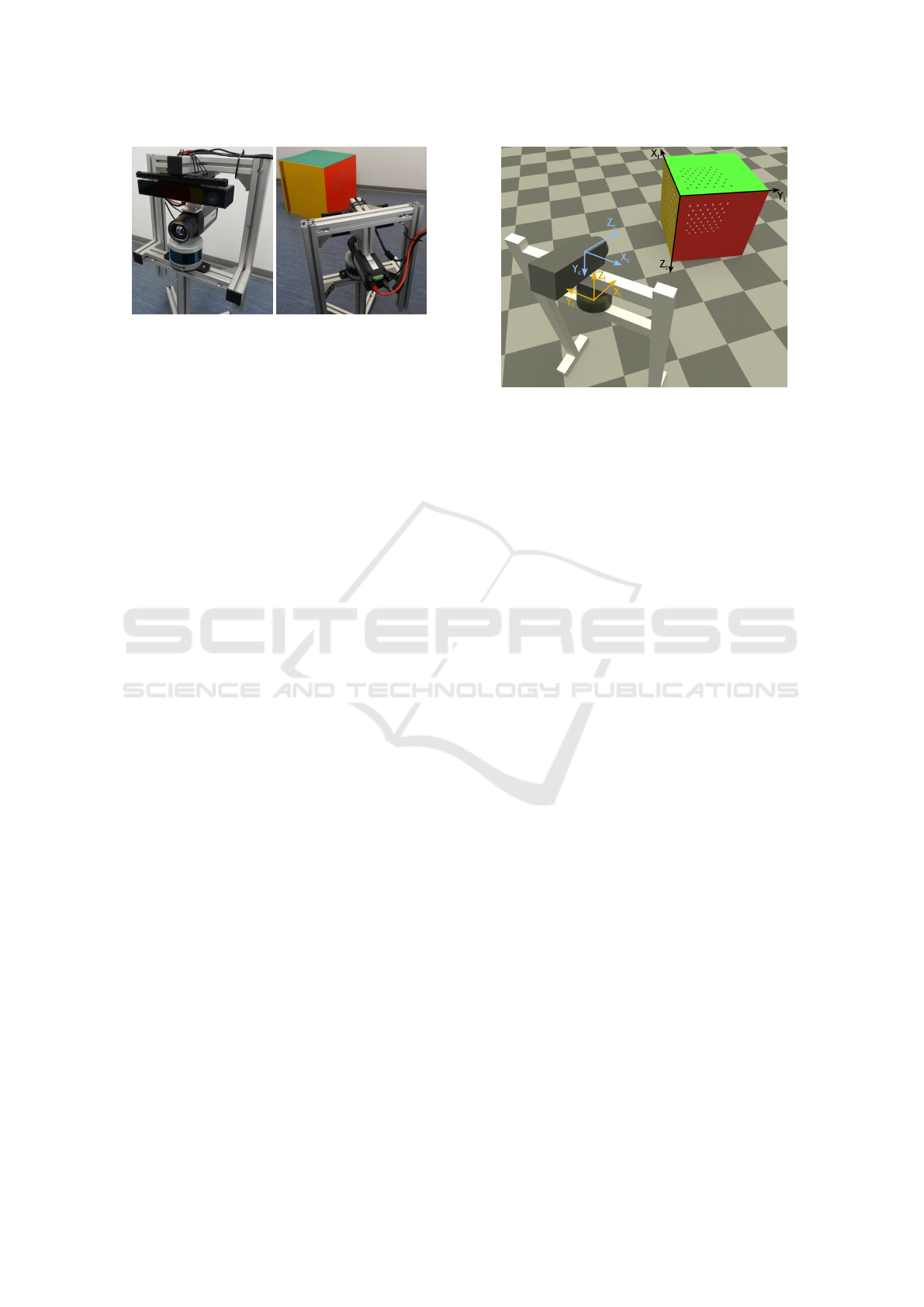
(a) Sensor stack (b) Calibration setup

Figure 2: Sensors used during calibration: (a) sensor setup

consisting of LRF (bottom), TIC (center) and Kinect v2

(top, not used in this work), and (b) calibration setup be-

tween the sensor stack and the calibration target.

a short explanation at this place. The general cali-

bration setup is depicted in Figure 2(b). Let us de-

ﬁne different coordinate frames (X, Y, Z) by using the

indices c, l and t in order to express quantities with

respect to the camera, laser and trihedron coordinate

systems (see also Figure 3). The extrinsic calibration

between the LRF and the TIC is deﬁned by a (3 × 3)

rotation matrix R

and a (3 × 1) translation vec-

tor t

. This transformation can also be expressed as

a transformation from the laser coordinate frame to

the trihedron coordinate frame (R

, t

) = (R

−1

, t

−1

followed by a transformation to the camera coordi-

nate frame (R

, t

). A 3D point p

with respect to

the laser coordinate frame can be projected onto the

TIC’s image plane using the pinhole camera model:









= K(R

+ t

), (1)

where [u v]

is a 2D point in the image plane scaled

by the factor s and K is the camera matrix containing

intrinsic calibration parameters.

In order to ﬁnd the individual geometric transfor-

mations, a common calibration target is needed. We

use a heated trihedron whose planes made of PVC

are orthogonally oriented. On each of these planes, a

pattern of small circles was created using aluminum-

containing spray. Observing these three planes with

the LRF allows to ﬁnd the transformation from the tri-

hedron coordinate frame to the laser coordinate frame

, t

). In the thermal image, the circles of the

patterns let us ﬁnd the corresponding transformation

from the trihedron coordinate frame to the camera co-

ordinate frame (R

, t

In the following subsections, we show how to ﬁnd

the initial transformations for the optimization proce-

dure and how to reﬁne the calibration parameters.

Figure 3: Model of the calibration setup: Coordinate frames

of the TIC (X

, Y

, Z

), of the LRF (X

, Y

, Z

) as well as of

the calibration trihedron (X

, Y

, Z

). On each plane of the

trihedron, there is a pattern consisting of small circles.

3.1 Finding Initial Transformations

Finding the rotation matrix R

and translation vec-

tor t

that transform 3D points with respect to the

trihedron coordinate frame to 3D points with respect

to the laser coordinate frame is accomplished using

the plane equations for each of the trihedron’s planes.

In the following explanations, we utilize a superscript

notation using i, j and k (or variations) to refer to in-

dividual laser-camera data pairs (i ∈ 1, 2, ..., I), indi-

vidual planes ( j ∈ 1, 2, 3) and individual 3D points

(k ∈ 1, 2, ..., K) lying in a plane. The plane equa-

tions are acquired with the help of a RANSAC-based

plane extraction method. Each of the planes detected

by the LRF is deﬁned by a unit normal vector

( j)

and

a distance d

( j)

from the laser coordinate frame’s ori-

gin to the plane. The corresponding plane equation

is p

( j)

− d

( j)

= 0, where p

( j)

is an arbitrary point

lying in the jth plane.

The individual columns of R

depict the planes’

unit normal vectors

( j)

with the result that:







ˆn

(1)

l,x

ˆn

(2)

l,x

ˆn

(3)

l,x

ˆn

(1)

l,y

ˆn

(2)

l,y

ˆn

(3)

l,y

ˆn

(1)

l,z

ˆn

(2)

l,z

ˆn

(3)

l,z







. (2)

The translation vector t

can be calculated multiply-

ing R

with the vector of plane distances:

= R







(1)

(2)

(3)







. (3)

This vector points from the laser coordinate frame’s

origin to the trihedron’s corner, which is also the ori-

gin of the trihedron coordinate frame.

ICINCO 2016 - 13th International Conference on Informatics in Control, Automation and Robotics

160

The determination of rotation matrix R

and

translation vector t

that transform 3D points with re-

spect to the trihedron coordinate frame to 3D points

with respect to the camera coordinate frame is quite

similar to the procedure described above. Using the

circle grid patterns, we ﬁnd the rotation matrices

and translation vectors for transforming the individ-

ual pattern coordinate frames to the camera coordi-

nate frame. These matrices and vectors can then be re-

lated to the trihedron coordinate frame. The columns

of R

, just like for the laser transformation, are the

planes’ unit normal vectors, i.e. the third column r

( j)

of the rotation matrix found for each pattern/plane

j ∈ {1, 2, 3}:

(1)

(2)

(3)

. (4)

The translation vector t

that points from the cam-

era coordinate frame’s origin to the trihedron’s origin

can be calculated with the help of one of the pattern-

camera transformations by shifting the pattern’s ori-

gin to the trihedron’s origin.

3.2 Reﬁning Calibration Parameters

A reﬁnement of the calibration parameters can be ac-

complished by matching the laser points lying in the

trihedron’s planes into the plane equations estimated

based on the thermal image data. Hence, we try to

ﬁnd R

and t

that satisfy the Hesse normal form of

each trihedron’s plane. This can be expressed as an

optimization problem of the following form:

argmin

∑

i=1

∑

j=1

∑

k=1



(i, j)

(i, j,k)

+ t

) − d

(i, j)



(5)

where K is the total number of points detected by the

LRF in one speciﬁc plane j and data pair i, and I is

the total number of laser-camera data pairs taken. A

solution for this non-linear least squares problem can

be found using the Levenberg-Marquardt algorithm.

4 HANDLING OF

MISINTERPRETATIONS

Most misinterpretations in thermal images originate

from an unknown emissivity ε, which is a surface-

speciﬁc property dependent especially on the type of

surface material and the TIC’s viewing angle. The

viewing angle is the angle between the camera’s opti-

cal axis and the surface normal of the regarded point.

According to (Martiny et al., 1996), the signal mea-

sured by the TIC can be expressed as:

sum

= εS

ob j

+ (1 − ε)S

amb

(6)

with

ob j

exp



ob j



− F

(7)

and

amb

exp



amb



− F

, (8)

if the the atmospheric amount of radiation power is

neglected. In Equation 6, S

sum

, S

ob j

and S

amb

repre-

sent output signals measured per image pixel. Ac-

cording to the subscripts, they depict the total out-

put signal, the output signal corresponding to the re-

garded object’s radiation power and the output signal

corresponding to the reﬂected ambience’s radiation

power. In Equations 7 and 8, T

ob j

and T

amb

are the

true object/ambient temperatures, while R, B and F

are camera-speciﬁc parameters provided by the TIC’s

manufacturer. From Equation 6, it can be seen that the

higher the emissivity value, the smaller the inﬂuence

of ambient reﬂections on the thermal image.

Since in mobile robot exploration a preparation of

the environment before measurement (e.g. using high

emissivity coatings) is not applicable, we developed

two methods for improving the interpretation of ther-

mal images regarding unknown surface emissivities

and thermal reﬂections.

4.1 Estimation of Unknown Emissivities

This section refers to our previous work in (Zeise

et al., 2015), where we showed the feasibility of

temperature correction for surfaces regarded from a

known viewing angle. In our approach, we estimated

improved surface temperature values of metal and di-

electric surface points exploiting the different emis-

sivity characteristics of metals and dielectrics at a

varying viewing angle.

In general, the approach divides into two subrou-

tines. The ﬁrst step is to determine the regarded sur-

face point’s material class, i.e. metal or dielectric.

This can be done by observing one individual point’s

output signal at different viewing angles. As we de-

rived from Equation 6, the total output signal depends

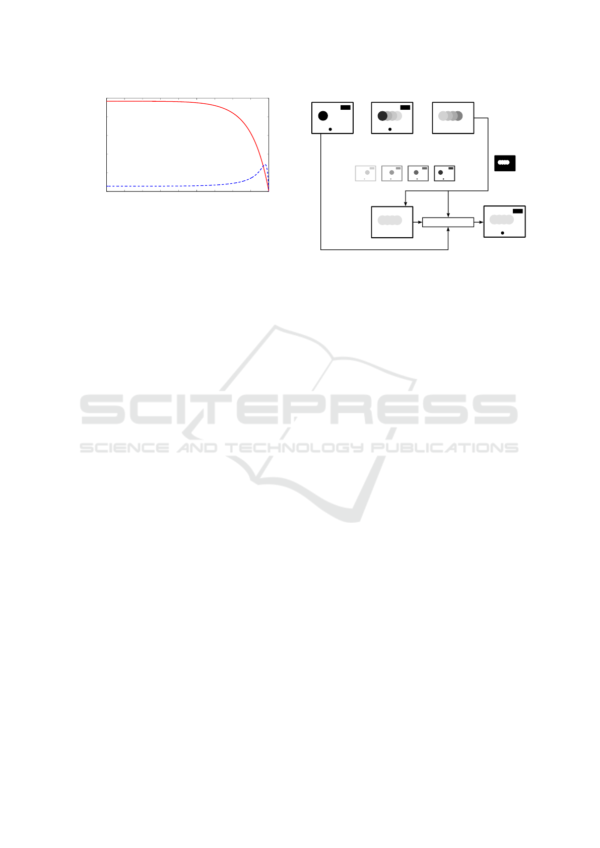
linearly on the emissivity. Due to the fact that the

emissivity in general shows a qualitative behavior as

depicted in Figure 4, it is sufﬁcient to investigate the

individual pixel’s output signal in order to assign one

of the properties metal or dielectric to the point.

Temperature Correction and Reﬂection Removal in Thermal Images using 3D Temperature Mapping

161

0 10 20 30 40 50 60 70 80 90

0.2

0.4

0.6

0.8

Viewing angle in °

Directional emissivity

Figure 4: Qualitative comparison of metal (blue, dashed

line) and dielectric (red, solid line) emissivity characteris-

tics depending on the viewing angle.

The second step is to estimate improved temper-

ature values for each individual point on the surface.

This can be done using non-linear least squares opti-

mization minimizing the error between the measured

output signals at different viewing angles and theoret-

ically calculated output signals that depend mostly on

emissivity. Equations describing emissivity as a func-

tion of the viewing angle can be found in the litera-

ture, e.g. in (Howell et al., 2011). The minimization

is performed as:

argmin

∑

z=1



− S

(p)



, (9)

where p = {n, k, T

ob j

, T

amb

} is the set of parameters to

be found. In this set of parameters, the refractive in-

dex n and the extinction coefﬁcient k, together with

the corresponding viewing angle, describe the graph

of emissivity ε. The signals S

and S

represent mea-

sured/calculated values at Z different viewing angles.

In order to use our approach, some assumptions

have to be made. On the one hand, both the surface

temperature T

ob j

and the ambient temperature T

amb

are assumed to be unknown but constant. On the

other hand, T

ob j

must be higher than T

amb

. Since the

assumption that T

amb

= const. is in conﬂict with the

occurrence of thermal reﬂections, it is necessary to

identify and remove them before correcting the sur-

face temperatures.

4.2 Thermal Reﬂection Removal

Handling of thermal reﬂections can be accomplished

by using background subtraction. The relation of

temperature values and 3D information can be used

to investigate temperature changes of speciﬁc surface

points. For our investigations, we assume a static en-

vironment, which implies that the temperatures of the

regarded surfaces do not change over time. Hence,

if an individual surface point’s measured temperature

does not change when the camera moves, it means

– =

+ + +

I(t) I

avg1

(t) I

diﬀ

(t)

I(t-3)I(t-4) I(t-2) I(t-1)

...

avg2

(t)

Inverted

Reﬂection

Area Mask

= 0.30

= 0.15

res

(t)

Image generation

Figure 5: Illustration of the reﬂection removal procedure:

Weighted moving averages of thermal images are used to

handle reﬂections (see the text for a detailed description).

that the temperature is mostly the temperature of the

surface itself. In contrast, a changing temperature of

one speciﬁc surface point implies a superposition of

the actual surface temperature and a thermal reﬂec-

tion.

In Figure 5, our approach to thermal reﬂection re-

moval is illustrated. Let I(t), I(t − 1), ..., I(t − n) be a

set of registered thermal images of a static scene taken

from different points of view. The weighted moving

average I

avg

(t) at time t can be calculated using the

following equation:

avg

(t) = wI(t) + (1 − w)I

avg

(t − 1), (10)

where w is a weighting factor inﬂuencing the impor-

tance of the latest image I(t). A high value of w means

more inﬂuence of the current image on the moving

average. We use this factor to create two individual

moving averages: In the ﬁrst, I

avg1

(t), the latest ther-

mal image has a major inﬂuence on the average im-

age. Subtracting this average image from the current

thermal image gives us I

di f f

(t) that can be regarded

as a reﬂection mask. Every pixel in I

di f f

(t) that is not

zero/white represents a potential reﬂection. The sec-

ond moving average image, I

avg2

(t), is created using

a smaller weighting factor in combination with the re-

ﬂection mask. Masking out the non-reﬂective pixels

allows to generate an image that contains only reﬂec-

tive pixels. In contrast to the mask itself and the ﬁrst

average image, the reﬂective areas in I

avg2

(t) are very

smooth. This smooth image is then used to ﬁll the re-

ﬂective areas during image generation. Depending on

whether the regarded pixel was marked as reﬂective

or not in the reﬂection mask, the image generation ei-

ther uses data from I

avg2

(t) or from I(t) to generate

the resulting image I

res

(t).

ICINCO 2016 - 13th International Conference on Informatics in Control, Automation and Robotics

162

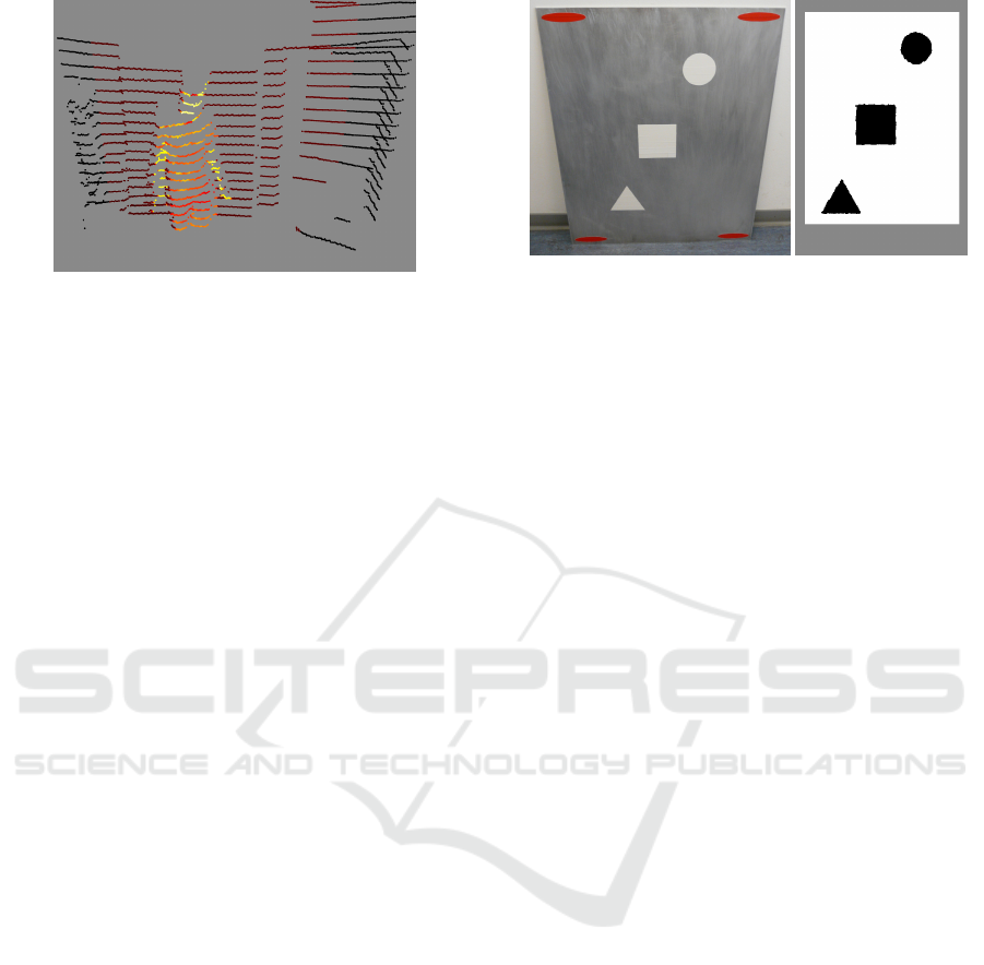
Figure 6: Mapping results: False-colored point cloud show-

ing a person standing in front of a cupboard.

5 EVALUATION

The evaluation was performed using the Velodyne

Puck LRF and the Flir A655sc TIC. The LRF pro-

vides dense, horizontal scans with a ﬁeld of view of

360

◦

, while the vertical ﬁeld of view is only 30

◦

con-

sisting of 16 scan lines. The TIC has a spatial resolu-

tion of 640 x 480 pixels, working in a spectral range

between 7.5 µm and 14 µm. The camera’s ﬁeld of

view is 45

◦

x 34

◦

5.1 Laser-Camera Calibration and

Temperature Mapping

As stated in Section 3, the intrinsic calibration param-

eters for the LRF were taken as provided by the man-

ufacturer. The intrinsics of the TIC were estimated

using a heated aluminum plate covered with squares

made of aluminum and PVC. The parameter estima-

tion was performed using standard computer vision

algorithms (Zhang, 2000).

The laser-camera calibration can be assessed look-

ing at the temperature mapping results (Figure 6).

Since the vertically sparse point cloud complicates an

objective temperature mapping evaluation, we do not

provide information on the reprojection error.

5.2 Temperature Correction

The temperature correction algorithm was evalu-

ated using the heated, low-emissive aluminum plate

(56 cm x 70 cm) depicted in Figure 7(a). On the plate,

there are several stripes of high-emissive duct tape

forming shapes of a triangle, a square and a circle.

The aim of this evaluation is to ﬁrst identify the re-

garded material class for every individual pixel in the

thermal image. After that, we use this information to

(a) Reﬂective plate (b) Material classiﬁ-

cation result

Figure 7: Reﬂective plate: (a) RGB image of the low-

emissive aluminum plate and (b) the result of the mate-

rial classiﬁcation procedure (white areas = metal, black ar-

eas = dielectric, gray areas = not speciﬁed).

estimate improved values of the surface points’ tem-

peratures.

We took more than 50 laser-camera data pairs of

the heated plate while continuously increasing the

sensors’ viewing angle. Using the four elliptic tags

near the corners of the plate, we were able to reg-

ister consecutive images. In addition, we used the

LRF’s 3D point cloud data to calculate every individ-

ual pixel’s viewing angle.

The results of the material classiﬁcation are de-

picted in Figure 7(b). The algorithm distinguishes be-

tween metal and dielectric points by adding up the

differences between consecutive measurements taken

from increasing viewing angles. If the resulting value

is greater than zero, the algorithm tags the surface

point as metal, otherwise as dielectric.

The temperature correction is performed for ev-

ery individual surface point. Depending on the ma-

terial class, parameters n, k, T

ob j

and T

amb

are es-

timated using non-linear optimization. To solve the

least squares minimization problem, we make use of

the Levenberg-Marquardt algorithm.

The plate’s true surface temperature was deter-

mined using an additional surface thermometer. On

the metal areas, we measured a temperature of about

317 K. The dielectric shapes had a slightly lower tem-

perature of about 316 K. The direction of reﬂection

was covered with a wall having a temperature of about

295 K, ensuring a constant ambient temperature T

amb

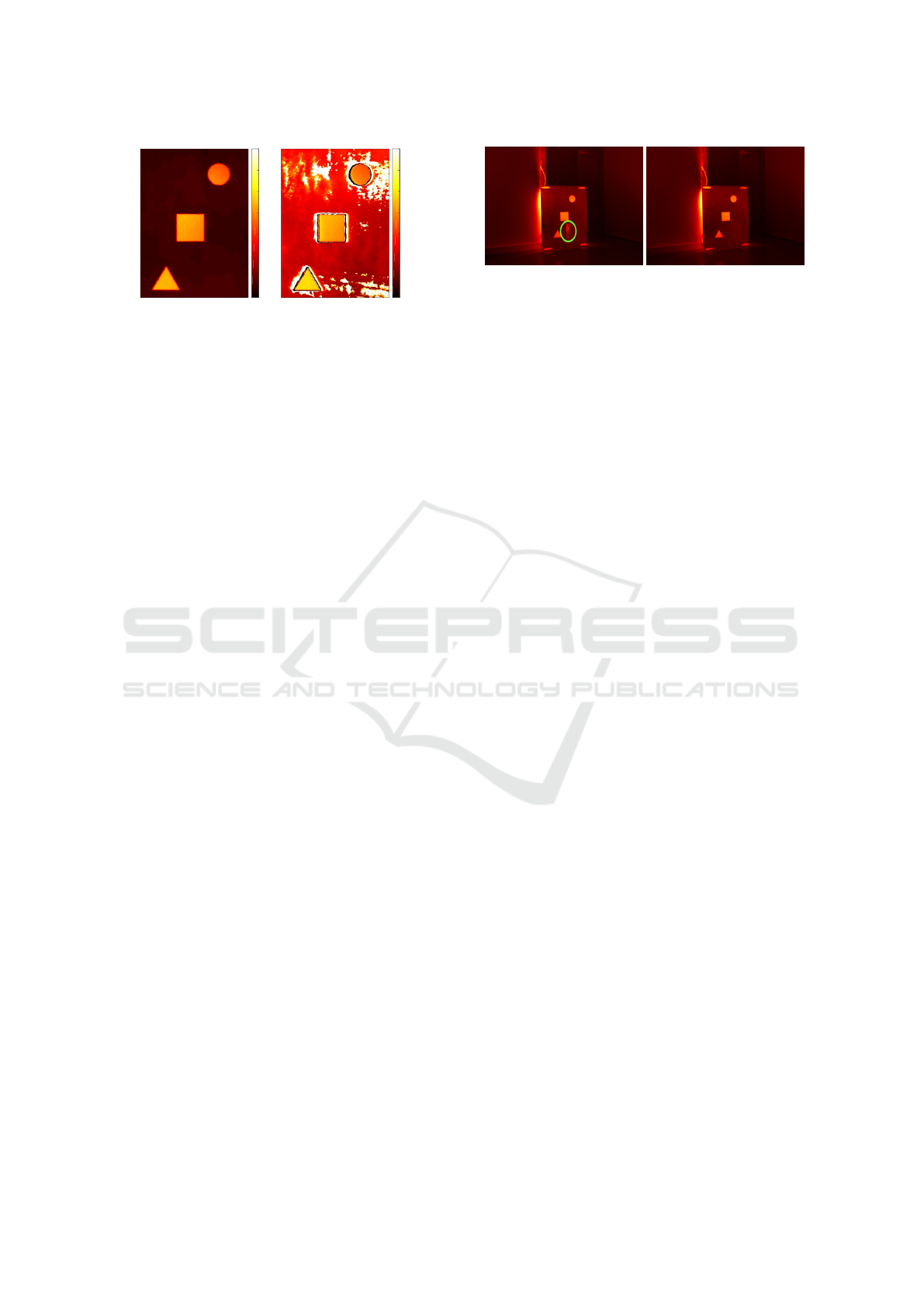
The optimization results are depicted in Figure 8.

The aluminum temperatures in the original thermal

image are obviously misinterpreted. While in the

original image (i.e. without taking emissivity into

account) the metal surface had an average tempera-

ture of about 297 K, our method was able to correct

this value to about 305 K for most of the metal sur-

Temperature Correction and Reﬂection Removal in Thermal Images using 3D Temperature Mapping

163

Temperature in K

295

300

305

310

315

320

325

330

(a) Original thermal im-

age

Temperature in K

295

300

305

310

315

320

325

330

(b) Processed thermal

image

Figure 8: Temperature correction results (false-colored): (a)

Original thermal image with metal areas interpreted as too

cold (dark) and (b) the corrected image with improved tem-

perature interpretations.

face points. Due to a high emissivity of the dielectric

points, there are almost no misinterpretations in these

areas. Hence, the corrected dielectric temperatures

are nearly the same as the ones originally measured.

While in the border areas between dielectric and

metal points we expected wrong estimations, the re-

sults regarding the metal areas are in need of improve-

ment. This can mostly be traced back to the wave-

length dependency of the optical constants n and k (as

introduced in Section 4.1). Since all measurements

taken by the TIC take into account the whole wave-

length spectrum between 7.5 µm and 14 µm, n and

k, which can vary at different wavelengths, cannot

be unambiguously determined. This is also the rea-

son for erroneously estimated high temperature val-

ues represented by the bright areas in Figure 8(b).

5.3 Reﬂection Detection and Removal

To evaluate the capabilities of our reﬂection removal

approach, we used the same aluminum plate as for the

temperature correction experiment. As stated before,

the bare aluminum surface is highly reﬂective to ther-

mal radiation. We placed a can ﬁlled with hot water

(approx. 350 K) in the direction of reﬂection. We cre-

ated a dataset, taking thermal images while simulta-

neously changing the camera’s point of view. Apply-

ing our algorithm to this dataset leads to the results

depicted in Figure 9.

The resulting image shows that the thermal reﬂec-

tion could be most widely removed. During our ex-

periments, we noticed a thin, black borderline in the

corrected image at the edge of the aluminum plate.

We trace this back to the fact that our algorithm cuts

out the plate in order to ensure an accurate image

registration. Assuming a complete 3D environment

model in our future research, these borderlines will

not be present anymore.

(a) Original image (b) Resulting image

Figure 9: Reﬂection removal result for an exemplary dataset

(false-colored): (a) shows the original image containing a

reﬂection of a can (marked by the ellipse), while (b) depicts

the processed image without reﬂection.

A possible shortcoming of our approach is that

only moving reﬂections can be detected at the mo-

ment. For later stages of our work, one solution for

this could be to keep track of reﬂections as soon as

they were detected.

6 CONCLUSION AND FUTURE

WORK

In this work, we faced the problem of handling misin-

terpretations in thermal images making use of spatial

knowledge of the regarded scene. We acquired in-

formation of the camera’s viewing angle by using a

rigidly mounted sensor setup consisting of a TIC and

a LRF, which we extrinsically calibrated with the help

of a heated calibration trihedron.

We ﬁrst presented an approach that – using the

emissivity’s viewing angle dependency – is able to

improve temperature measurements of surfaces with

unknown emissivity values. Our method showed

good results in determining the material class (dielec-

tric/metal) of regarded surface points. While the gen-

eral functionality of the temperature correction was

demonstrated, the results are yet limited due to several

unsolved dependencies (e.g. wavelength-dependent

optical constants).

The second method presented deals with thermal

reﬂections. Exploiting the TIC’s varying viewing an-

gle, our algorithm based on background subtraction

was able to detect and remove reﬂections from the

images. Experiments showed that moving thermal re-

ﬂections could successfully be removed.

Future work will focus on integrating the pre-

sented approaches into a 3D simultaneous localiza-

tion and mapping (SLAM) algorithm. By doing this,

our algorithms will beneﬁt from the spatial knowl-

edge of the scene on the one hand, while enhancing

the generated environment model with improved tem-

perature mapping on the other hand. Additional effort

ICINCO 2016 - 13th International Conference on Informatics in Control, Automation and Robotics

164

can be spent on tuning the performance of the tem-

perature correction algorithm, e.g. by using a GPU

implementation.

ACKNOWLEDGEMENTS

This work has partly been supported within H2020-

ICT by the European Commission under grant agree-

ment number 645101 (SmokeBot).

REFERENCES

Agrawal, A., Raskar, R., Nayar, S. K., and Li, Y. (2005).

Removing photography artifacts using gradient pro-

jection and ﬂash-exposure sampling. ACM Trans.

Graph., 24(3):828–835.

Alba, M. I., Barazzetti, L., Scaioni, M., Rosina, E., and Pre-

vitali, M. (2011). Mapping infrared data on terrestrial

laser scanning 3D models of buildings. Remote Sens-

ing, 3(9):1847–1870.

Aziz, M. Z. and Mertsching, B. (2010). Survivor search

with autonomous UGVs using multimodal overt at-

tention. In IEEE Safety Security and Rescue Robotics,

pages 1–6, Bremen, Germany.

Borrmann, D., Elseberg, J., and Nüchter, A. (2013). Ther-

mal 3D mapping of building façades. In Lee, S., Cho,

H., Yoon, K.-J., and Lee, J., editors, Intelligent Au-

tonomous Systems 12, number 193 in Advances in

Intelligent Systems and Computing, pages 173–182.

Springer Berlin Heidelberg, Berlin, Heidelberg.

Criminisi, A., Kang, S. B., Swaminathan, R., Szeliski, R.,

and Anandan, P. (2005). Extracting layers and ana-

lyzing their specular properties using epipolar-plane-

image analysis. Computer Vision and Image Under-

standing, 97(1):51–85.

Farid, H. and Adelson, E. H. (1999). Separating reﬂections

and lighting using independent components analysis.

In IEEE Computer Society Conference on Computer

Vision and Pattern Recognition, volume 1, pages 262–

267, Fort Collins, CO, USA.

Gong, X., Lin, Y., and Liu, J. (2013). 3D LIDAR-camera

extrinsic calibration using an arbitrary trihedron. Sen-

sors, 13(2):1902–1918.

Howell, J. R., Siegel, R., and Mengüç, M. P. (2011). Ther-

mal radiation heat transfer. CRC Press, Boca Raton,

FL, USA, 5th edition.

Iuchi, T. and Furukawa, T. (2004). Some considerations

for a method that simultaneously measures the tem-

perature and emissivity of a metal in a high tem-

perature furnace. Review of Scientiﬁc Instruments,

75(12):5326–5332.

Iwasaki, Y., Kawata, S., and Nakamiya, T. (2013). Ve-

hicle detection even in poor visibility conditions us-

ing infrared thermal images and its application to road

trafﬁc ﬂow monitoring. In Sobh, T. and Elleithy, K.,

editors, Emerging Trends in Computing, Informatics,

Systems Sciences, and Engineering, number 151 in

Lecture Notes in Electrical Engineering, pages 997–

1009. Springer New York, New York, NY, USA.

Li, Y. and Brown, M. S. (2013). Exploiting reﬂection

change for automatic reﬂection removal. In IEEE

International Conference on Computer Vision, pages

2432–2439, Sydney, Australia.

Litwa, M. (2010). Inﬂuence of angle of view on tempera-

ture measurements using thermovision camera. IEEE

Sensors Journal, 10(10):1552–1554.

Martiny, M., Schiele, R., Gritsch, M., Schulz, A., and Wit-

tig, S. (1996). In situ calibration for quantitative

infrared thermography. In International Conference

on Quantitative InfraRed Thermography, pages 3–8,

Stuttgart, Germany.

Muniz, P. R., Cani, S. P. N., and Magalhães, R. d. S. (2014).

Inﬂuence of ﬁeld of view of thermal imagers and an-

gle of view on temperature measurements by infrared

thermovision. IEEE Sensors Journal, 14(3):729–733.

Pandey, G., McBride, J., Savarese, S., and Eustice, R.

(2010). Extrinsic calibration of a 3D laser scanner and

an omnidirectional camera. IFAC Proceedings Vol-

umes, 43(16):336 – 341.

Planas-Cuchi, E., Chatris, J. M., López, C., and Arnaldos, J.

(2003). Determination of ﬂame emissivity in hydro-

carbon pool ﬁres using infrared thermography. Fire

Technology, 39(3):261–273.

Schechner, Y. Y., Kiryati, N., and Basri, R. (2000). Sepa-

ration of transparent layers using focus. International

Journal of Computer Vision, 39(1):25–39.

Szeliski, R., Avidan, S., and Anandan, P. (2000). Layer

extraction from multiple images containing reﬂections

and transparency. In IEEE Conference on Computer

Vision and Pattern Recognition, volume 1, pages 246–

253, Hilton Head Island, SC, USA.

Vidas, S., Moghadam, P., and Bosse, M. (2013). 3D ther-

mal mapping of building interiors using an RGB-D

and thermal camera. In IEEE International Confer-

ence on Robotics and Automation, pages 2311–2318,

Karlsruhe, Germany.

Vollmer, M., Henke, S., Karstädt, D., Möllmann, K. P.,

and Pinno, F. (2004). Identiﬁcation and suppression

of thermal reﬂections in infrared thermal imaging. In

InfraMation Proceedings, volume 5, pages 287–298,

Las Vegas, NV, USA.

Zeise, B., Kleinschmidt, S. P., and Wagner, B. (2015). Im-

proving the interpretation of thermal images with the

aid of emissivity’s angular dependency. In IEEE Inter-

national Symposium on Safety, Security, and Rescue

Robotics, pages 1–8, West Lafayette, IN, USA.

Zhang, Q. and Pless, R. (2004). Extrinsic calibration of a

camera and laser range ﬁnder (improves camera cali-

bration). In IEEE/RSJ International Conference on In-

telligent Robots and Systems, volume 3, pages 2301–

2306, Sendai, Japan.

Zhang, Z. (2000). A ﬂexible new technique for camera cal-

ibration. IEEE Transactions on Pattern Analysis and

Machine Intelligence, 22(11):1330–1334.

Temperature Correction and Reﬂection Removal in Thermal Images using 3D Temperature Mapping

165