
Synthetic Workload Generation of Broadcast Related HEVC Stream
Decoding for Resource Constrained Systems
Hashan Roshantha Mendis and Leandro Soares Indrusiak
Real-time Systems Group, Department of Computer Science, University of York, York, U.K.
Keywords:
HEVC, Decoding, Workload Characterisation, Synthetic Workload Generation.
Abstract:
Performance evaluation of platform resource management protocols, require realistic workload models as in-
put to obtain reliable, accurate results. This is particularly important for workloads with large variations, such
as video streams generated by advanced encoders using complex coding tools. In the modern High Efficiency
Video Coding (HEVC) standard, a frame is logically subdivided into rectangular coding units. This work
presents synthetic HEVC decoding workload generation algorithms classified at the frame and coding unit
levels, where a group of pictures is considered as a directed acyclic graph based taskset. Video streams are
encoded using a minimum number of reference frames, compatible with low-memory decoders. Characteristic
data from several HEVC video streams, is extracted to analyse inter-frame dependency patterns, reference data
volume, frame/coding unit decoding times and other coding unit properties. Histograms are used to analyse
their statistical characteristics and to fit to known theoretical probability density functions. Statistical proper-
ties of the analysed video streams are integrated into two novel algorithms, that can be used to synthetically
generate HEVC decoding workloads, with realistic dependency patterns and frame-level properties.
1 INTRODUCTION
HEVC (H.265) as well as its predecessor, H.264,
both utilise advanced video coding techniques to ef-
ficiently compress highly dynamic and diverse video
streams. Advanced compression techniques such as
the use of hierarchical B-frame structures (Sullivan
et al., 2012), random-access profiles (Chi et al., 2013)
and scene-change detection (Eom et al., 2015), makes
video decoding workloads highly variable and com-
plex. As video streaming workloads become more
sophisticated, efficient platform resource manage-
ment mechanisms and optimised scheduling of tasks
and are required at the decoder to optimise perfor-
mance. Input workloads highly influence the sim-
ulation based evaluation of these resource manage-
ment protocols, therefore it is crucial to achieve an
analytical, tractable and realistic, model or abstrac-
tion of the actual application. For example, in re-
search where workload properties such as task ex-
ecution costs are assumed to be Uniform/Gaussian
distributed (e.g.(Yuan and Nahrstedt, 2002; Mendis
et al., 2015)), the performance evaluation might sig-
nificantly deviate from the results obtained using a re-
alistic workload with a non-uniform distribution (e.g.
skewed/long-tailed).
HEVC frames are logically structured as coding
tree blocks (CTB) and each CTB is recursively sub-
partitioned into coding units (CU) in a quad-tree man-
ner (illustrated in Figure 1). The CU defines a re-
gion sharing the same prediction mode (e.g., intra and
inter). This work, analyses traces from real HEVC
decoding workloads at the group of pictures (GoP),
frame and CU levels. Workload generation algo-
rithms are presented, that use statistical distribution
models that closely represent video decoding work-
load characteristics. Frame decoding time is derived
in a bottom-up manner by utilising CU-level charac-
teristics.
Novel Contributions: This work introduces algo-
rithms, that can be used to generate directed acyclic
graph (DAG) based HEVC decoding workloads, with
statistical properties closely matching real HEVC
video streams. These synthetically generated, abstract
workloads can then valuable in simulation-based de-
sign space exploration research (such as in (Mendis
et al., 2015; Kreku et al., 2010)), to investigate timing
and performance properties more accurately. To our
knowledge this is the first work to characterise HEVC
decoding workloads at the block-level as well as cap-
turing the properties of GoP-level task graphs depen-
dency patterns, for different types of video streams.
52
Mendis, H. and Indrusiak, L.
Synthetic Workload Generation of Broadcast Related HEVC Stream Decoding for Resource Constrained Systems.
DOI: 10.5220/0005953200520064
In Proceedings of the 13th International Joint Conference on e-Business and Telecommunications (ICETE 2016) - Volume 5: SIGMAP, pages 52-64
ISBN: 978-989-758-196-0
Copyright
c
2016 by SCITEPRESS – Science and Technology Publications, Lda. All rights reserved

64x64
32x32
16x16
8x8
CU-level information extraction:
* Prediction type (I/P/B/Skip)
* Size distribution
* Decoding execution cost
* Reference data dependency
I
P
B B
GoP-level characteristics:
* Distribution of P, B frames
* Hierarchical B-frame structure
* Scene change rate
* Inter-prediction reference distance
Inter-task communication:
* Frame-level reference data volume
* Memory read/write volume
I
P
B B
GoP
0
Sequence of open GoPs within the video stream
I
P
B B
GoP
1
I
P
B B
GoP
2
I
P
B B
GoP
3
C
0
C
1
C
2
C
3
e
0
e
1
e
2
e
3
e
4
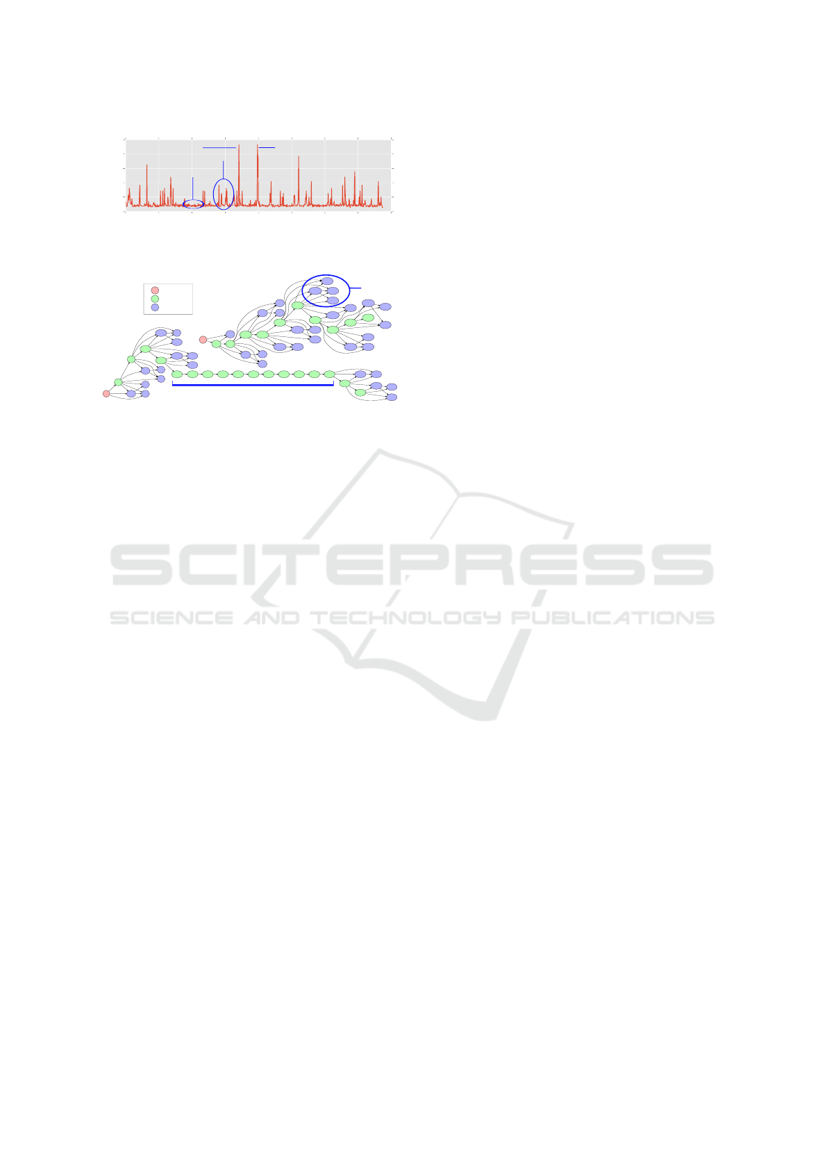
Figure 1: Task-graph based HEVC decoding workload.
Workload characterisation at different levels: taskset (GoP),
task (frame) and inter-task communication (reference data).
A group of pictures (GoP), represented via a
DAG based application model is shown in Figure 1.
There are essentially three kinds of frames in a GoP:
I-frames (intra-predicted), P-frames (uni-directional,
inter-predicted) and B-frames (bi-directional, inter-
predicted). Inter-predicted, P and B frames use ref-
erence data from other frames in the GoP to construct
the current frame. In this work, a task-graph (TG)
refers to the graph derived from the GoP structure,
where nodes in a TG refers to HEVC frame decoding
tasks and edges in a graph represents inter-prediction
frame data-dependencies. For example, the weight
of edge P ← I represent the overall decoded I-frame
data that is referenced by the P-frame. Video decod-
ing workloads are increasingly dynamic with highly
varying frame decoding execution costs and depen-
dency relationships based on the temporal and spatial
characteristics of the video streams. Most specially in
HEVC each inter-predicted frame can have up to 16
reference frames. Hence for example in a 35 frame
GoP, there could be up to 35×16 edges in the TG and
buffer requirements would vary greatly as well.
This work explores the following workloads char-
acteristics of different video streams:
• Taskset/GoP Characteristics: number of P and
B frames in a GoP, TG dependency characteris-
tics, scene-changes, reference frame distribution.
• Task/Frame and CU Level Characteristics: de-
coding time and frame-to-CU relationship analy-
sis, CU-size and type distributions.
• Inter-task Communication Characteristics:
reference data volume per frame/CU-type (i.e.
task communication traffic) and encoded frame
size analysis (i.e. task memory read traffic)
2 RELATED WORK
In previous research, video decoding workloads have
primarily been characterised at the functional level.
Functional computation units of the video decoder
such as entropy decoding, motion compensation, fil-
tering, inverse quantisation etc. are identified and
considered as tasks with data dependencies. A com-
prehensive discussion of the computation cost of the
HEVC decoding functional units on ARM and x86
platforms have been given by Bossen et al. (Bossen
et al., 2012). They show that motion compensation
and entropy decoding dominate the decoding time of
a random-access video stream. Holliman et al. (Hol-
liman and Chen, 2003), analyse MPEG-2 and H.264
decoding workloads from a system architecture per-
spective by investigating how CPU branch predic-
tions, cache and main memory hierarchy effects ex-
ecution time. An abstract workload model of a paral-
lel H.264 decoder is introduced in the MCSL bench-
mark framework (Liu et al., 2011). They specify the
decoder functional unit execution cost and inter-task
communication traffic as actual traces obtained from
recorded real video streams as well as data derived
from statistical properties of trace-data. However,
their workload properties such as execution cost, re-
lease patterns, inter-task traffic volumes are assumed
to be Gaussian distributed, which may not be accurate
with the real underlying distribution.
Video decoding workloads have also been anal-
ysed at the data-level, where a task can be consid-
ered as decoding video streams at at different lev-
els of granularity (e.g. GoP/frame/slice/block etc.).
The data communication between the tasks represent
reference data. Encoded frame sizes have been as-
sumed to follow a Gamma, Lognormal or Weibull dis-
tribution (Mashat, 1999; Krunz et al., 1995). Tanwir
et al.(Tanwir and Perros, 2013) in their survey pa-
per, show that wavelet-based models offer a reason-
able compromise between complexity and accuracy
to model frame sizes, and the model prediction re-
sults can vary significantly based on the type of en-
coding. Frame decoding time is assumed to have a
linear relationship with the frame size (Bavier et al.,
1998). However, Isovic et al. (Isovic et al., 2003)
show that there is a large variance in the decoding
time for the same frame size. Roitzsch et al. (Roitzsch
and Pohlack, 2006) estimates the total decoding time
of a frame by adding macroblock and frame-level
metrics into video stream headers at the encoder-end.
In more recent work, Benmoussa et al. (Benmoussa
et al., 2015) uses a linear regression model to illustrate
the relationship between bit rate and frame decoding
time. High variability in decoding times are seen for
Synthetic Workload Generation of Broadcast Related HEVC Stream Decoding for Resource Constrained Systems
53

FastFurous5
LionWildlife Football
ObamaSpeech BigBuckBunny ColouredNoise
Figure 2: Video sequence snapshots.
I/P/B frame-types due to different coding tools in
each type and memory access patterns (Alvarez et al.,
2005). Therefore, classification based on frame type
need to be addressed in the model in order to obtain an
accurate representation of video decoding workloads.
To our knowledge this is the first work to present
characterisation and analysis of HEVC decoding at
the CU-level, for different types of video streams. Un-
like previous work, we analyse the reference frame
patterns within a GoP as well as frame/block level de-
coding times. We provide algorithms that construct
HEVC GoPs and frames using a bottom-up method-
ology by using characteristics derived at the CU-level.
3 VIDEO SEQUENCE AND
CODEC TOOL SELECTION
The video sequences under investigation has been
chosen to represent varying levels of spatial and tem-
poral video characteristics. Below are the video se-
quences selected for this study (snapshots presented
in Figure 2):
• FastFurious5 (Action, 720p, 30fps, 15mins):
Heavy panning/camera movement, frequent scene
changes.
• LionWildlife (Documentary, 720p, 30fps,
15mins): Natural scenery, medium move-
ment scenes, fade in/out, grayscale to colour
transitions.
• Football (Sport, 720p, 30fps, 15mins): camera
view mostly on field, camera panning, occasional
close-ups on players/spectators. Large amounts of
common single colour background, combined text
and video.
• ObamaSpeech (Speech footage, 720p, 24fps,
10mins): Constant, non-uniform background;
uni-camera and single person perspective, head-
/shoulder movement.
• BigBuckBunny (CGI/Animation, 480p, 25fps,
9mins): Wide range of colours, moderate scene
changes.
• ColouredNoise (Pseudo Random coloured pix-
els, 720p, 25fps, 10mins): Low compression, use-
ful for analysing worst-case characteristics of a
codec.
3.1 Encoder and Decoder Settings
The video streams were encoded using the open
source x265 encoder (v1.7) (Multicoreware, 2015).
x265 has shown to produce a good balance between
compression efficiency and quality (Zach and Slan-
ina, 2014; Naccari et al., 2015), by incorporating sev-
eral advanced coding features such as adaptive, hi-
erarchical B-frame sequences. The default settings
of x265 (Multicoreware, 2015) are complimented
with additional settings (Listing 1), to suit resource-
constrained decoding platforms (e.g. set-top box,
smart phone), targeted at broadcast/video streaming
applications. Main memory data traffic of dependent
picture buffer (DPB) access has shown to impact real-
time display of high definition (HD) video sequences
(Soares et al., 2013). Furthermore, multiple refer-
ence frames can linearly increase the memory usage
of the decoder (Saponara et al., 2004). Therefore,
inter-prediction has been restricted to 1 forward and 2
backward references. Higher number of B-frames in
a GoP offers better compression but decreases inter-
frame compression and quality (Wu et al., 2005). To
strike a balance, the encoder was configured to use a
maximum of 4 contiguous B-frames.
Listing 1: x265-encoder and OpenHEVC-decoder
command-line arguments.
Encoder:
x2 65 -- i npu t vid_ raw . yuv - o v i d_ enc . bin -I 35
-- b - a da pt 2 - - b fr ame s 4 --no - we i gh tp --no -
we i gh tb
-- no - ope n - g op --b - i nt ra -- r ef 2 -- csv - log - l ev el
2 -- csv v i d_s tat s . cs v - - log - le vel 4
Decoder:
oh ev c -i v id_ en c . bi n - f 1 -o vid_ dec . yuv - p 1 -n
Key-frames (random access-points in the
video) provide the ability to move (e.g. fast-
forward/pause/rewind) within a video stream. x265
by default treats all I-frames as key-frames if the
closed-GoP (self-contained/independent GoPs) set-
ting is chosen. Closed-GoPs offer less compression
than open-GoPs, but reduce error propagation during
data losses, hence more suited for broadcast video.
To ensure a balance between compression and
random-access precision, maximum I-frame interval
of 35 frames was chosen. Weighted prediction
was disabled to increase decoder performance and
B-frames were allowed to have intra-coded blocks in
order to be efficient during high motion/scene-change
SIGMAP 2016 - International Conference on Signal Processing and Multimedia Applications
54
0 100 200 300 400 500 600 700 800
GoP index
0
1
2
3
4
5
Inter-predicted
frames ratio (P/B)
Football goal scored
Goal replay
Ball goes out of field,
play restart
Normal
game play
Figure 3: Ratio of P:B frames within a GoP for (Football
video).
b28
b5
B14
b15
b13
b7
b1
B10 b9
b11
b3
I0
P4
B2
P27
P30
B29
B32
b31
b33
P12
P16
P17 P18 P19 P20
P34
P23 P24
P8
B6
P25 P26P21 P22
b28
b26
b23
b21
b5
b7
B12 b11
b1
b3
b9
b16
I0
P2
B31
b30
b32
P10 P13
B8
b14
P17
B15
b18
b19
B20
P22
P33
P34
P6
B4
B27
P29
B24
P25
Hierarchical
B-Frames
Long sequence of P-frames
(high motion video sequence)
I-frame
B-frame
P-frame
Figure 4: Example structure of a GoP (from BigBuck-
Bunny). Top: low number of P-frames, Bottom: high num-
ber of P-frames. (NB: edges and nodes are unweighted).
sequences.
Decoding execution trace data was obtained us-
ing the open source, OpenHEVC (Opensource, 2015;
Hamidouche et al., 2014) decoder with the minimal
settings (Listing 1). In order to eliminate any inter-
thread communication and synchronisation latencies
which might affect decoding time data capture, for
this work, multi-threading has been disabled. The
platform used for decoding was a laptop with Intel
Core i7-4510U 2.00GHz CPU, 4MB L3-cache and
8GB of DDR3 RAM.
4 GoP STRUCTURE MODEL
The GoP structure is directly related to the scene
changes and motion in the video. For example, the ra-
tio of the number of P and B frames per GoP (denoted
as P/B ratio) of the Football changes with respect
to high-motion scenes/scene-changes (Figure 3). We
measure the scene change rate as 1/GoP
di f f
, where
GoP
di f f
refers to the mean number of GoPs between
scene change events. The scene change rate in each
tested video stream is given in Table 1. This met-
ric gives a notion of how often the GoP structure
changes with respect to time. FastFurious5 has the
highest scene change rate while the Football video has
the lowest. P-frames give higher compression than
I-frames, hence during scene changes, the x265 en-
coder increases the P/B ratio, whilst keeping the GoP
length constant. Figure 4 shows two example GoPs
from the BigBuckBunny video; the bottom GoP refers
a high-motion scene (more P-frames).
4.1 Distribution of Different Frame
Types
The number of P and B frames in a GoP for each video
sequence is shown as a histogram in Figure 5. The
number of P-frames in a GoP (denoted nP) is mod-
elled as an exponentiated-Weibull (exp-Weibull) dis-
tribution (Mudholkar et al., 1995), where the proba-
bility density function (PDF) of the exp-Weibull dis-
tribution is given as Eq. 1 with shape parameters a
and c. Additional scale and location parameters de-
fines the relative size and position of the PDF; they
are specific to the statistics package used (i.e. SciPy).
f (x) = ac (1 −exp −x
c
)
a−1
exp−x
c
x
c−1
(1)
Gamma and Gumbel PDFs provided inaccurate
fits to the distributions, motivating the use of exp-
Weibull distribution due to its long-tail, right-skewed
density and flexibility in shape. From Figure 5, it
is clear that most of the video sequences fit the exp-
Weibull distribution except for the case of Coloured-
Noise, where no variation in the number of P or B
frames is seen. Due to the constant GoP length N,
the number of B-frames nB = (N − 1) − nP, giving
us an inverted distribution. For low-motion videos
such as ObamaSpeech with no scene changes (Ta-
ble 1), the P,B distributions show less variation and
do not overlap; furthermore high values of c and a
are seen. Video sequences with large variation in mo-
tion, long-tailed distributions are seen (e.g. BugBuck-
Bunny), with a low c,a.
4.2 Contiguous B-frames & Reference
Distance
The maximum number of contiguous B-frames
(nB
max
) in a GoP is an encoder parameter, which is
set to 4 in our study. Figure 6 shows the proportion of
different contiguous B-frames in a GoP. Low-motion
videos (e.g. ObamaSpeech), show a high level of
contiguous B-frames, while high motion videos (e.g.
FastFurious5), the proportions are uniform. The pro-
portion of contiguous B-frames have a direct impact
to the reference distance of a frame. Reference dis-
tance (RFD) is the absolute difference between the
GoP index of the current frame and its parent/depen-
dent frame(s). Larger reference distances correlate
with higher contiguous B-frames in a GoP. Higher av-
erage reference distances in a video stream, means the
decoder has to keep a decoded frame longer in the
DPB, which would result in high buffer occupancy
and hence a larger main memory requirement.
Generally, P-frames do not refer to B-frames and
if the encoder is restricted to have only 1 reference
Synthetic Workload Generation of Broadcast Related HEVC Stream Decoding for Resource Constrained Systems
55
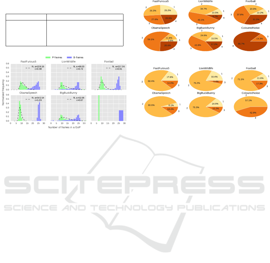
Table 1: Scene change rate for all video sequences. GoP
di f f
refers to the mean number of GoPs between scene-changes.
VidName Scene change rate (1/GoP
di f f
)
FastFurious5 0.45
BigBuckBunny 0.30
LionWildlife 0.20
Football 0.05
ObamaSpeech 0.00
Figure 5: P,B frame histogram for all video sequences (dis-
tributions fitted to the exp-Weibull PDF with shape param-
eters (a,c), location=0, scale=1.5).
frame for the forward direction, then a P frame refers
to the closest previous I/P frame. B-frames referred to
past and future I/P/B frames with a RFD characteris-
tic as shown in Figure 7. A highest B-frame RFD of 3
is seen as we restricted the maximum number of con-
tiguous B-frames in the GoP to 4. Further analysis
showed that a contiguous sequence of B-frames re-
ferred only to I/P-frames in close temporal proximity;
therefore long edges in the task graph are not present.
A correlation exists between the RFD ratios shown
in Figure 7 and the number of contiguous B-frames
shown in Figure 6. For example, less than 10% of
of contiguous B-frames in LionWildlife are of size 4,
which leads to a very low number of frames having a
RFD of 3.
4.3 GoP Structure Generation
Construction of a synthetic GoP structure can be done
in two stages as per Algorithm. 1. Firstly, a GoP
sequence (in temporal decoding order) is generated,
taking into account the exp-Weibull distributed P,B
frames. The position of the B-frames within the GoP
are uniformly distributed, but the selection of con-
tiguous B-frame sizes are derived from the ratio rela-
tionships observed from the trace results (Figure 6).
Lines 12-19 generate B-frame groups (Hierarchical
B-frames) and inject them at random positions in the
GoP. In phase II of the algorithm, each inter-predicted
frame is assigned reference frames as per the anal-
ysis in Section 4.2. The number of reference frame
Figure 6: Number of contiguous B-frames in a GoP.
Figure 7: Reference distances for B-frames in different
video sequences.
per temporal direction is an algorithm parameter. P
frames are assigned the immediate previous I/P frame
in the GoP. B-frames are assigned multiple refer-
ence frames (past and future) as per the RFD ratios
seen in Figure 7. Lines 28, 34 and 36 derive possi-
ble and legal reference frames within the GoP. The
RAND.CHOICE function, generates a random sample
from the given possible reference frame set, according
to the specified probabilities (derived from the distri-
butions).
The parameter N in Algorithm 1 can be varied to
obtain different GoP lengths. nBmax and W
p
can be
varied to obtain different numbers of B and P frames
within a GoP. rB
f wd
max
,rB
bwd
max
and rP
f wd
max
can be used to
provide more reference frames to P and B frames, this
would in turn increase the number of edges in the TG.
vs
prob
r f d
is representative of the length of the edges in
the TG and also gives a notion of the number of pos-
sible reference frames for a B-frame.
5 DERIVING A FRAME-LEVEL
TASK MODEL
HEVC frames are logically partitioned into CTBs and
each CTB is sub-partitioned into CUs (Figure 1). The
objective of this work is to analyse the video prop-
erties at the CU granularity in order to understand
and derive a frame decoding model. For example,
when modelling an I-frame, a higher proportion of
smaller CU sizes may need to be used, while hav-
ing no P/B/Skip-CUs. A fine-grain workload charac-
terisation can also facilitate exploration of CU/wave-
SIGMAP 2016 - International Conference on Signal Processing and Multimedia Applications
56
front/tile level task models as seen in (Roitzsch and
Pohlack, 2006; Chi et al., 2012).
5.1 CU Sizes, Types and Decoding Time
HEVC CUs can be of the size 64x64, 32x32, 16x16,
8x8, 4x4 (intra only) and can use either intra (I-
CU) or inter (P/B/Skip-CU) prediction. I-CUs refer
to other CUs within the same frame and P/B/Skip-
CUs refer to CUs in other frames. Skip-CUs are
those which do not have a residual or motion vector,
hence a reference-CU is copied directly, resulting in
reduced computation complexity at the decoder and
higher compression efficiency. Analysis of the CUs
by size and type is necessary to derive a coarse-grain
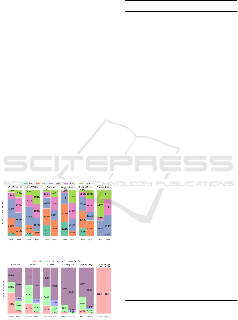
frame-level model. Figure 8 shows that intra and in-
ter predicted frame types differ significantly in the us-
age of different CU sizes. There are a higher number
of smaller CUs in detailed scene background videos
(e.g.ObamaSpeech and Football) than others because.
Overall, 64x64 CUs are least used than other sizes,
however inter-frames seem to use significantly more
64x64 CUs than intra-frames. The encoder has failed
to use small CU sizes for the ColouredNoise video.
As seen in Figure 9, except for ColouredNoise, all
other videos contain a large proportion of Skip-CUs.
The number of intra-predicted CUs (I-CU) seem to
be higher in video sequences with high-motion. The
inverse is true of Skip-CUs; for example in Oba-
Figure 8: Proportion of CU sizes within each video se-
quence (per Intra/Inter frame type).
Figure 9: Proportion of CU types within each video se-
quence (per Inter frame type).
Algorithm 1: Pseudo-code for GoP structure con-
struction.
1 Phase I - Construct GoP sequence
/* Parameter definition */
2 N = GoP length;
3 nB
max
= max. sequential B-frames;
4 assert((N − 1)%(nB
max
+ 1) == 0), validate parameters;
5 nP
min
= (N − 1)/(nB
max
+ 1);
6 nP
max
= (N − 1), max. P-frames;
/* Contiguous B-frame probs. - Figure 6 */
7 B
prob
seq
= [p
0
..p
(nB
max
)
];
/* exp. Weibull distributed num. P,B-frames */
8 W
p
= exp-Weibull PDF shape params: a, c, scale,loc
nP = EXPWEIBULL(W
p
).SAMPLE(nP
min
, nP
max
);
9 nB = (N −1) − nP;
10 nB
sizes
= [1..nB
max
], contiguous B-fr lengths;
/* main data structures */
11 B
f r
= {} /* hash table of positions and B-frame
numbers */
12 GOP
f r
= “I” + (“P” ∗ nP);
/* get contigous B-fr positions in the GoP */
13 while
∑
B
f r
.values() < nB do
14 pos = RAND.CHOICE([1..nP], prob=’UNIFORM’);
15 tmpB
f r
= RAND.CHOICE(nB
size
,prob=B
prob
seq
);
16 if (B
f r
[pos].value + tmpB
f r
) <= nB
max
then
17 B
f r
[pos]+ = tmpB
f r
;
18 end
19 end
20 GOP
f r
← B
f r
/* Put B-frames into GoP */
21 Phase II - Construct GoP frame references;
/* maximum frame references */
22 rB
f wd
max
,rB
bwd
max
= max. forward and backward B-frame refs.;
23 rP
f wd
max
= max. forward P-frame refs.;
24 vs
prob
r f d
: ref. dist. ratios;
/* hash table of inter-fr references */
25 f r
re f s
= {}
26 for f r
ix
, f r ∈ GOP
f r
do
/* P-frames depend on prev. I/P frs */
27 if f r == “P” then
28 r
all f wd
POCs
= GOP
f r
[POC < f r
ix
∩ (r
d
≤
r
max
d
) ∩ ¬“B”];
29 re f s
f wd
= RAND.CHOICE(r
all f wd
POCs
,size = rP
f wd
max
,
30 prob=vs
prob
r f d
);
31 f r
re f s
[ f r
ix
] = re f s
f wd
32 else if f r == “B” then
/* B-fr depend on prev/future I/P/B frs */
33 r
all f wd
POCs
= GOP
f r
[POC < f r
ix
∩ (r
d
≤ r
max
d
)];
34 r
all bwd
POCs
= GOP
f r
[POC > f r
ix
∩ (r
d
≤ r
max
d
)];
35 re f s
f wd
= RAND.CHOICE(r
all f wd
POCs
,size = rB
f wd
max
,
36 prob=vs
prob
r f d
);
37 re f s
bwd
= RAND.CHOICE(r
all bwd
POCs
,size = rB
bwd
max
,
38 prob=vs
prob
r f d
);
39 f r
re f s
[ f r
ix
] = {re f s
f wd
,re f s
bwd
};
40
41 end
maSpeech, the amount of Skip-CUs are between 80-
93%. Overall the number of P-CUs seem to be 2-
3 times the amount of B-CUs, and P-frames have
a higher amount of I-CUs than B-frames. The en-
Synthetic Workload Generation of Broadcast Related HEVC Stream Decoding for Resource Constrained Systems
57
coder has failed to use inter-prediction to compress
the ColouredNoise, where 99% of the video has been
coded using intra-CUs. BigBuckBunny has lower
amount of frame data because of the lower video res-
olution (480p).
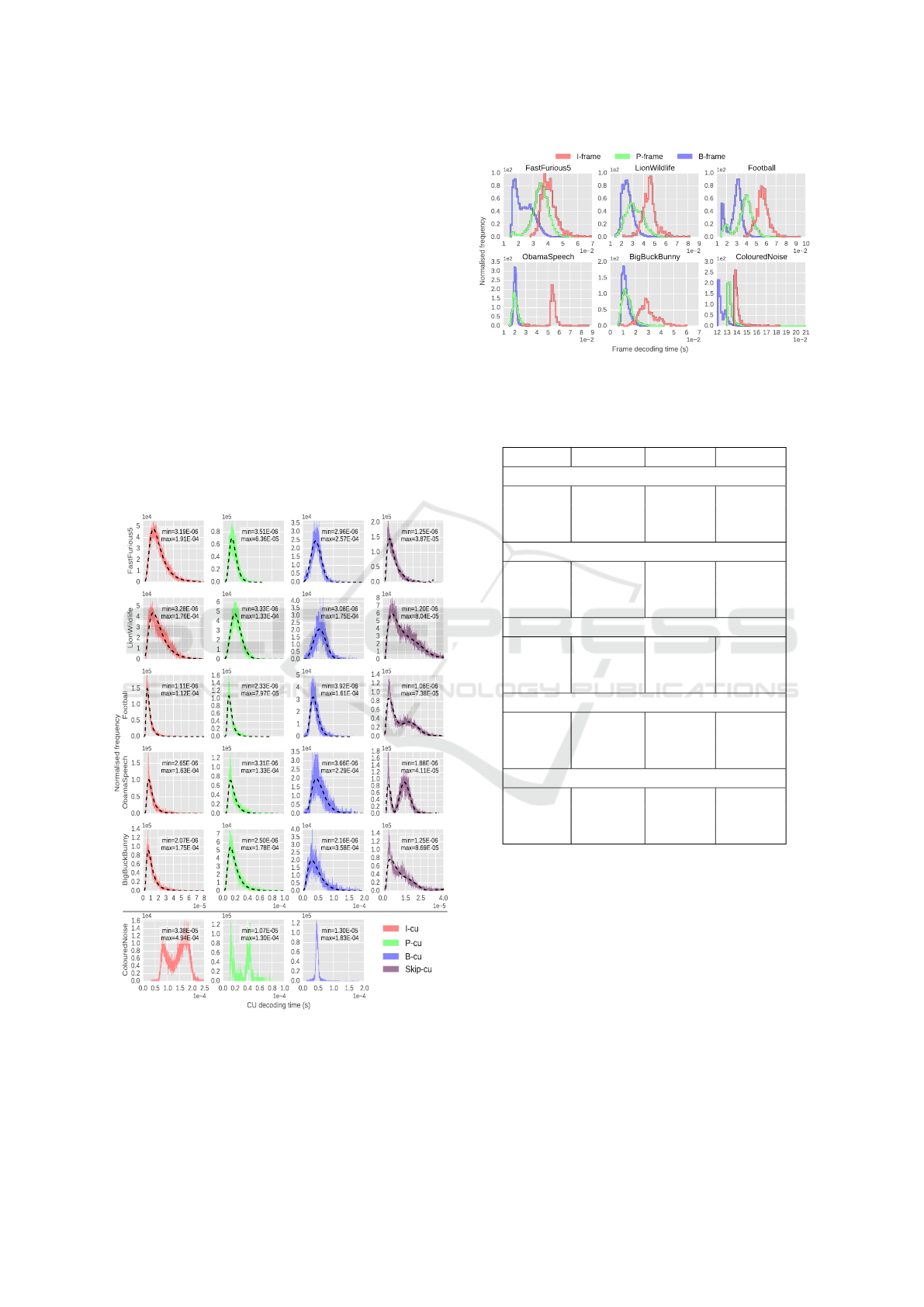
The distributions of CU-level decoding time are
given in Figure 10. I,P and B-CUs are fitted with
a exp-Weibull distribution (parameters given in Ta-
ble 2). Skip-CUs could belong to either P or B frames,
and could have 1 or 2 reference CUs; hence, the Skip-
CU decoding times appear to be multi-modal. They
are fitted with a high-order polynomial function (co-
efficients given in Table 3). The large coefficient val-
ues in the model presents a risk of over fitting the data;
however, we do not use the model to predict the de-
coding times, but randomly sample the distribution to
generate new workloads. As future work, regularisa-
tion can be used to prevent over fitting.
High B-CU decoding times are due to complex
transformations, in bidirectional inter-prediction. B-
Figure 10: Normalised CU-level decoding time histogram
per video sequence. I/P/B-CUs distributions fitted to a exp-
Weibull PDF (dashed line; parameters given in Table 2);
polynomial function fitted to Skip-CUs (parameters given
in Table 3). (NB: Subfigures use different scales, share axes
and distribution tails are cropped in order to assist visuali-
sation).
Figure 11: Normalised frame-level decoding time distribu-
tion histogram for each video sequence.
Table 2: I/P/B-CU decoding time distribution, exp-Weibull
fit shape parameters. (default location=0).
CU type a c scale
FastFurious5
I-CU 1.77E+01 6.56E-01 3.05E-06
P-CU 7.47 1.28 8.42E-06
B-CU 1.38 2.55 4.51E-05
LionWildlife
I-CU 9.24 7.43E-01 5.06E-06
P-CU 3.29 1.57 1.58E-05
B-CU 1.38 2.78 5.78E-05
Football
I-CU 2.87E+03 3.21E-01 1.02E-08
P-CU 9.12E+02 4.46E-01 1.44E-07
B-CU 7.13 1.35 1.99E-05
ObamaSpeech
I-CU 1.23E+03 3.25E-01 2.09E-08
P-CU 8.07E+02 3.93E-01 1.08E-07
B-CU 6.54 1.14 2.49E-05
BigBuckBunny
I-CU 6.56E+02 3.08E-01 1.93E-08
P-CU 3.47E+01 5.62E-01 1.49E-06
B-CU 4.74 9.47E-01 1.91E-05
CUs decoding times are about 2-3 times larger than
I and P-CUs. The CU decoding time is dependent on
the CU-size and content of the video sequence. This is
evident in the Football B-CU decoding times, where
compared to others has a lower variance in decoding
times, because of a higher proportion of inter-frame
8x8 CUs in the video stream. Furthermore, in Li-
onWildlife a high amount of 16x16,32x32,64x64 CU
sizes is seen, which could give rise to larger CU de-
coding times. Larger CU-sizes could lead to higher
decoding times due to bottlenecks at the memory sub-
systems (Kim et al., 2012). A trend can be seen in
the I-CU decoding time and the exp-Weibull shape
parameters; where high-motion, high scene-change
videos such as FastFurious5 and LionWildlife have
SIGMAP 2016 - International Conference on Signal Processing and Multimedia Applications
58
a lower a and higher c, leading to wider distribu-
tions. Overall Skip-CUs have the lowest decoding
time compared with the other CU-types.
The I-CU decoding time in ColouredNoise gave
the highest execution time out of all the videos; giv-
ing an observed worst-case CU decoding time of
4.94×10
−4
s. Football shows the lowest Skip-CU de-
coding time (1.08×10
−6
s), which indicates that de-
coding CUs can have two orders of magnitude vari-
ation, depending on the type of video and CU-type
and size. The CU-level decoding time data in Fig-
ure 10 correlates with the frame-level decoding time
shown in Figure 11. Overall in every video stream,
t
I
> t
P
> t
B
where the terms t
I
, t
P
and t
B
denote I,P,B
frame decoding times. This is mainly due to the num-
ber of Skip-CUs in a frame. E.g. a B-frame primarily
contains Skip-CUs (Figure 9), and Skip-CUs decod-
ing times are lower than other CU types, resulting in
relatively lower overall B-frame decoding times. In
ObamaSpeech, I-frame decoding is approx. 2-3 times
larger than P,B-frame decoding. In FastFurious5 there
is low variation between average P and I frame de-
coding times, this is because 45% of P-frame CUs
are intra-coded. As expected it takes about 2-3 times
longer to decode ColouredNoise when compared to
the other streams, because about 99% of the stream
consists of I-CUs.
5.2 Inter-task Communication Volume
In Section 4.2 the inter-frame dependency pattern in a
GoP was discussed. This section investigates the vol-
ume of reference data required for inter-prediction,
which is essentially the weight of each arc in the
GoP-level TG. Apart from reference frame-data, the
encoded frame also needs to be loaded from main
memory in order to perform the decoding operations;
hence this data traffic also forms part of the commu-
nication volume in the application.
The reference data is the pixel data of a decoded
frame; the maximum amount of data a P-frame can
reference is ( f r
size
= (h×w)×bpp), where h and w rep-
resents the frame dimensions and bpp is bytes per
pixel. For B-frames this upper bound is doubled due
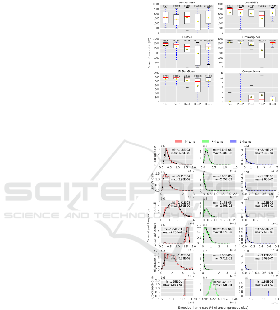
to bi-directional prediction. Figure 12 shows the dis-
tribution of reference data categorised by direction of
reference; for example P ← I refers to the data ref-
erenced by a P-frame from an I-frame in the GoP.
Considering the distributions and their sample sizes
for each video stream, overall all inter-frames have
a preferred reference probability of: p
I
> p
P
> p
B
,
where for example p
I
denotes the probability of a
frame obtaining data from an I-frame. This observa-
tion is true because B-frames have the lowest decoded
Figure 12: Distribution of frame reference data for all video
sequences. E.g. P ← I refers to the data referenced by a
P-frame from an I-frame. Sample-size of the distribution
given as n.
Figure 13: Distribution of frame compression ratio (en-
coded frame size as a % of the uncompressed frame size).
Distribution fitted to Exp-Weibull PDF (dashed-line, pa-
rameters given in Table 4). (NB: Subfigures use different
scales in order to assist visualisation).
frame data accuracy due to bi-directional prediction,
and I-frames have the highest accuracy due only us-
ing intra-prediction. In a synthetic frame-level task
generator, probabilities of reference frame selection
is only required when the encoder allows the use of
Synthetic Workload Generation of Broadcast Related HEVC Stream Decoding for Resource Constrained Systems
59

more than 1 reference frame per direction. Further
observations showed that when considering the total
amount of referenced data per frame-type, B-frames
referenced twice the amount of data than P-frames.
The reference data distributions are highly depen-
dent on the reference frame distance (Figure 7), the
number of contiguous B-frames (Figure 6) and the
distribution of frame types (Figure 5) in a GoP. This is
also the reason for the wide variation of reference data
in the B ← P distribution. The data traffic variation
seems to be higher in videos with high rate of scene-
change (e.g. FastFurious5), while the mean amount
of data volume is higher in largely static videos (e.g.
ObamaSpeech). ColouredNoise has very low refer-
ence data because a majority of the CUs are I-CUs.
The distribution of frame compression ratio are
given in Figure 13; this data represents the size of
an encoded frame. The distributions are fitted with
a exp-Weibull distribution (parameters given in Ta-
ble 4). Unlike in (Krunz et al., 1995) where a Log-
normal distribution gave the best fit for frame-size,
a right skewed distribution such as ObamaSpeech,
does not fit a Lognormal distribution well. Overall,
s
I
> s
P
> s
B
, where s
I
,s
P
,s
B
denote I/P/B encoded
frame sizes. However, the long-tailed distributions
tell us that there may be extreme-case scenarios where
this may not always be true (further verified in (Iso-
vic et al., 2003)). It can be observed that variation in
the distribution is relative to the motion/scene-change
rate of the video streams. Low-motion videos such as
ObamaSpeech have a much lower encoded P/B frame
size than high-motion videos. The distributions cor-
relate with the distribution of CU-sizes and CU-types
in a frame (Figure 8 and Figure 9). B-frame sizes
have very long-tailed distributions compared to I or
P-frames due to the variation in the number of Skip-
CUs in the frame; because Skip-CUs do not contain
a residual, the amount of data encoded is relatively
small. In general I-frame sizes have less variation
than inter-predicted frames.
5.3 Frame-level Task Generation
Algorithm 2 illustrates the frame-generation algo-
rithm pseudocode. The algorithm builds up the frame-
level task in a hierarchical bottom-up manner, by first
iterating through each CTU in the frame (line 13) and
then constructing a set of CUs per CTU (lines 15-32).
The frame decoding time is calculated as the sum-
mation of the CU decoding time (C
dt
) of all CUs in
the frame. Videos of different resolutions can be gen-
erated by changing the N
CTU
parameter accordingly;
h,w in line 2 is the resolution of the video. For each
CU in a CTU an appropriate value for the CU-type
Algorithm 2: Pseudo-code for frame construction, us-
ing CU-level properties.
/* Parameter definition */
1 CTU
px
max
= 64×64;
2 N
CTU
= (h×w)/CTU
px
max
,number of CTUs per frame;
3 CU
sizes
= 64,32, 16, 8,4;
4 CU
p
size
= CU size probabilities per frame type - Figure 8;
5 CU
types
= {I-CU, P-CU, B-CU, Skip-CU};
6 CU
p
types
= CU type probabilities - Figure 9;
7 W
I
p
,W
P
p
,W
B
p
= expWeibull parameters: a, c, scale,loc;
8 p
skip
c
= Skip-CU polynomial coefficients;
9 dI
lim
CU
,dP
lim
CU
,dB
lim
CU
,dSkip
lim
CU
= min/max CU dec. cost;
/* Ref. frame selection params - Optional: if more
than 1 ref. frames per direction. */
10 f r
re f
= reference frames for current frame;
11 PB
r f
= Prob. of current fr referencing I/P/B frames;
/* Construct each CTU in the frame */
12 f r
CTUs
= /* empty CTU list in frame */
13 for each CTU ∈ [0..N
CTU
] do
14 px = 0;CTU
CUs
= {} /* init. data struct. */
/* get CU-level information */
15 while px < CTU
px
max
do
/* randomly select CU size */
16 C
s
= RAND.CHOICE(CU
sizes
,prob=C
p
s
);
17 if (px +C
s
) ≤ CTU
px
max
then
18 px+ = (C
s
)
2
;
/* randomly select CU type */
19 C
t
= RAND.CHOICE(CU
types
,prob=C
p
t
);
/* random dec. time per CU type */
20 if C
t
== “I-CU” then
21 C
dt
=
EXPWEIBULL(W
I
p
).SAMPLE(dI
lim
CU
);
22 else if C
t
== “P-CU” then
23 C
dt
=
EXPWEIBULL(W
P
p
).SAMPLE(dP
lim
CU
);
24 else if C
t
== “B-CU” then
25 C
dt
=
EXPWEIBULL(W
B
p
).SAMPLE(dB
lim
CU
);
26 else if C
t
== “Skip-CU ” then
27 C
dt
=
POLYNOMIAL(p
skip
c
).SAMPLE(dSkip
lim
CU
);
28 /* pick CU reference from reference
frame list */
29 C
r f
= RAND.CHOICE( f r
re f
,prob=PB
r f
);
/* append to CU list */
30 CU
in f o
= {C
s
,C
t
,C
dt
,C
r f
};
31 CTU
CUs
← CU
in f o
;
32 end
33 end
/* append to CTU list */
34 f r
CTUs
← CTU
CUs
;
35 end
(line 19), CU-size (line 16), CU decoding time (lines
20-27) and CU reference frame (line 28) is selected.
The selection process for these properties is facilitated
by the observations and derived PDFs at the CU/frame
level in Sections 5.1 and 5.2. A set of parameters
(lines 1-11) needs to be carefully chosen for the al-
gorithm, which are representative of the type of video
SIGMAP 2016 - International Conference on Signal Processing and Multimedia Applications
60

(e.g. high temporal activity with low number of fine-
grain visual details) one intends to generate.
5.3.1 Limitations of the Workload Model
The CU type and size ratios given in Figure 10, 9 are
mean results obtained at the stream-level for differ-
ent frame types. In order to obtain variation of these
proportions between different individual frames, we
vary each percentage value according to a normal dis-
tribution. For example, when generating a frame for
FastFurious5, rather than taking the same value (31%
probability) for a SkipCU, we sample a normal distri-
bution with µ = 0.31 and σ = 0.05. The σ value needs
to be high enough to add a certain level of variation
between different frames of the same video stream,
but not too high such that the original proportions will
be masked. In real video streams however, the varia-
tion between frames would be complex and would not
fit a theoretical distribution. A deeper analysis into
the distribution of the CU types and sizes of a distri-
bution of frames will need to be analysed, in order to
infer the variations between frames.
Secondly, the CU decoding time provided contain
latencies induced by the memory subsystems of the
platform. Hence, during our evaluation we noticed
the frame decoding time does not scale proportion-
ally to the number of different CUs. In order to ob-
tain a reasonable frame-level mode, the CU decod-
ing time model (Figure 10) needs to be scaled down.
Furthermore, the decoding time results shown in this
work are dependent on the decoder implementation
and our hardware architecture. The scale factors need
to be tuned appropriately to suit a platform with dif-
ferent memory and CPU characteristics. CUs that
require more memory transactions such as P/B/Skip
CUs would need to be scaled down more than I-CUs.
During evaluation of the generator we noticed a scale-
down factor of 0.02-0.03 for I/P/B-CUs and 0.002-
0.002 for Skip-CU decoding times gave satisfactory
results.
6 WORKLOAD GENERATOR
USAGE
As discussed in Section 1 the algorithms presented in
Algorithm 1 and 2 can be used in system-level sim-
ulations to facilitate evaluation of workload resource
management and scheduling techniques (e.g. (Mendis
et al., 2015; Kreku et al., 2010; Yuan and Nahrstedt,
2002)). For example in (Mendis et al., 2015), we see
a multi-stream video decoding application workload
that needs to be allocated to multiple processing el-
ements in order to maximise system utilisation. Fig-
ure 14 shows how the workload generators proposed
in this work can be integrated into system simulators.
The workload generators can be used to output task-
level information (e.g. dependency patterns, execu-
tion costs, communication costs, arrival times) of a
large quantity of video streams, into text-based data
files (e.g. XML/CSV format) and read back in by
the simulator to be used as input for system perfor-
mance evaluation. The bottom-up methodology fur-
ther adds flexibility into the framework, such that the
CU-level information can also be used to generate
HEVC tile/wave-front (Chi et al., 2013) based work-
loads, in a similar manner to generating frames.
As illustrated in Figure 14, a video stream can be
generated by generating multiple GoPs using Algo-
rithm 1. Within each GoP a frame can be generated
using Algorithm 2. Likewise, any number of video
streams can be synthetically generated and fed into
a simulator. The GoP/frame-level model parameters
(e.g. exp-Weibull PDF shape parameters, CU size/-
type ratios), should be selected based on the type of
video. Variations of videos can be generated by mix-
ing/adapting the model parameters. For example, a
high-motion video with a fine-detailed background
can be generated by using a high nP distribution sim-
ilar to LionWildlife (Figure 5) and using proportions
of CU-sizes similar to ObamaSpeech(Figure 8, high
4x4, 8x8 count).
Generate CUs
Generate Frame
Generate CUs
Generate Frame
Generate CUs
Generate Frame
Generate CUs
Generate Frame
N
Generate GoP
Generate CUs
Generate Frame
Generate CUs
Generate Frame
Generate CUs
Generate Frame
Generate CUs
Generate Frame
N
Generate GoP
Generate CUs
Generate Frame
Generate CUs
Generate Frame
Generate CUs
Generate Frame
Generate CUs
Generate Frame
N
Generate GoP
Generate CUs
Generate Frame
Generate CUs
Generate Frame
Generate CUs
Generate Frame
Generate CUs
Generate Frame
N
Generate GoP
Generate CUs
Generate Frame
Generate CUs
Generate Frame
Generate CUs
Generate Frame
Generate CTUs/CUs
Generate Frame
N
Generate GoP
(taskset with
dependencies)
M
Video stream (abstract workload)
System simulator
(e.g. multicore platform)
workload input
(pregenerated data files)
System evaluation
results
Scheduler
Resource manager
Processing elements
GoP/Frame/CU
generator
parameters
Proposed workload generator
Figure 14: Integration of the bottom-up workload generator
with a system simulator. (M=Number of GoPs).
Usage examples, implementation source code and
analysis data has been made open to the community
for reproducibility of the analyses/results and applica-
bility of the workload generation algorithms (Mendis,
2015).
7 EVALUATION
To evaluate the proposed video decoding workloads,
we synthetically generated 200 GoPs of the Lion-
Wildlife video stream and compared against the data
gathered from the real LionWildlife video. From Fig-
ure 15(a) we can see that the number of P-frames in
Synthetic Workload Generation of Broadcast Related HEVC Stream Decoding for Resource Constrained Systems
61
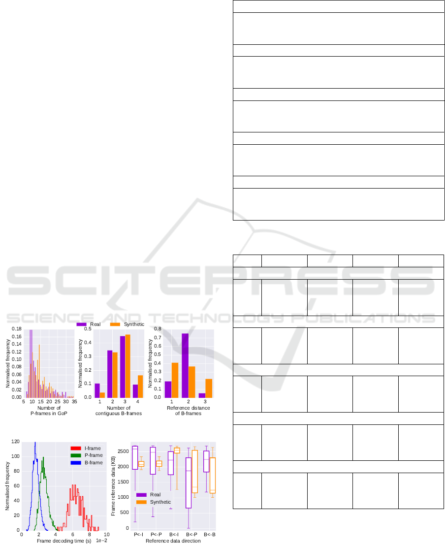
the generated GoPs follow a exp-Weibull distribution
as shown by the fit in Figure 5. However, the distri-
bution is slightly shifted to the right causing a higher
number of 4 contiguous B-frames which in turn af-
fects the reference distance ratios. A reference dis-
tance of 3 is still the lowest, similar to the real video
stream.
Figure 15(b)(left) shows the decoding time distri-
butions of the synthetically generated frames; these
need to be evaluated against the data given in Fig-
ure 11(LionWildlife). Due to inaccurate representa-
tion of the frame-level variations (Section 5.3.1), the
distribution of the frame decoding times generated do
not exactly follow the same shape as the real video
stream. However, we can see that the decoding times
are approximately in the same region for P and B
frames (i.e between 1.0 − 4.0×10
−2
s), which is ma-
jority of the video stream; and a slightly larger I-
frame decoding time (4.0 − 8.5×10
−2
s) can be seen.
The difference in decoding times between P and
B frames follow a similar trend to the real video
stream, as P-frame decoding times are overall larger
than B-frames. The generated frame decoding times
show a narrower spread of values than the real video
stream. We also evaluate the reference data volume
distributions between the synthetically generated and
real video stream. Figure 15(b)(right) shows that the
P ← I and P ← P show a narrower spread of data
volume than the real video stream. B ← I results are
higher than the real video and B ← B show a slightly
(a) GoP structure comparison: Left
(b) Frame characteristics comparison: Left
Figure 15: Comparison of GoP and frame-level characteris-
tics of a real vs. synthetically generated video stream.
Table 3: Skip-CU decoding time distribution, polynomial
fit coefficients.
FastFurious5, f(x)=
2.34×10
53
− 4.62×10
49
x +3.87×10
45
x
2
− 1.78×10
41
x
3
+
4.84×10
36
x
4
− 7.63×10
31
x
5
+ 5.82×10
26
x
6
+
4.03×10
20
x
7
− 4.09×10
16
x
8
+ 2.45×10
11
x
9
− 2.99×10
5
x
10
LionWildlife, f(x)=
−8.75×10
49
+ 3.92×10
46
x −7.60×10
42
x
2
+ 8.35×10
38
x
3
−
5.71×10
34
x
4
+ 2.52×10
30
x
5
− 7.21×10
25
x
6
+
1.30×10
21
x
7
− 1.38×10
16
x
8
+ 7.40×10
10
x
9
− 9.15×10
4
x
10
Football, f(x)=
−8.54×10
50
+ 3.41×10
47
x −5.87×10
43
x
2
+ 5.71×10
39
x
3
−
3.43×10
35
x
4
+ 1.32×10
31
x
5
− 3.24×10
26
x
6
+
4.90×10
21
x
7
− 4.22×10
16
x
8
+ 1.75×10
11
x
9
− 1.82×10
5
x
10
ObamaSpeech, f(x)=
5.45×10
52
− 4.99×10
48
x −3.55×10
44
x
2
+ 7.47×10
40
x
3
−
4.81×10
36
x
4
+ 1.65×10
32
x
5
− 3.32×10
27
x
6
+
3.93×10
22
x
7
− 2.61×10
17
x
8
+ 8.51×10
11
x
9
− 9.65×10
5
x
10
BigBuckBunny, f(x)=
−1.13×10
50
+ 5.22×10
46
x −1.04×10
43
x
2
+ 1.16×10
39
x
3
−
8.05×10
34
x
4
+ 3.58×10
30
x
5
− 1.03×10
26
x
6
+
1.84×10
21
x
7
− 1.92×10
16
x
8
+ 9.95×10
10
x
9
− 1.16×10
5
x
10
Table 4: Encoded frame size distributions, exp-Weibull fit
shape parameters.
Frame a c loc scale.
FastFurious5
I-Fr 4.76E+01 5.15E-01 5.81E-04 1.93E-04
P-Fr 1.57E+01 7.90E-01 2.71E-05 4.41E-04
B-Fr 1.29 7.38E-01 2.46E-05 3.08E-04
LionWildlife
I-Fr 1.31E+02 4.50E-01 0.00 1.52E-04
P-Fr 1.20E+01 5.07E-01 0.00 1.27E-04
B-Fr 1.17 7.79E-01 1.99E-05 2.47E-04
Football
I-Fr 6.05E-01 2.74E+00 2.74E-03 1.81E-02
P-Fr 4.15 9.49E-01 1.45E-04 1.56E-03
B-Fr 1.16 8.88E-01 1.92E-05 4.15E-04
ObamaSpeech
I-Fr 4.56E-01 6.21E+00 1.29E-02 3.69E-03
P-Fr 1.60 1.18E+00 3.79E-05 4.17E-04
B-Fr 8.45E+01 2.66E-01 2.31E-05 1.10E-07
BigBuckBunny
I-Fr 3.36 1.23 0.00 1.39E-02
P-Fr 5.51 4.59E-1 2.23E-05 1.70E-04
B-Fr 9.80E-01 7.34E-01 3.17E-05 2.57E-04
lower distribution. However the inter-quartiles of the
real and synthetic video distributions overlap, spe-
cially in the case of B ← P. These discrepancies are
also a result of the differences in B-frame reference
distances (Figure 15(a)(right)) and also the limitation
of getting an accurate view of the inter-frame CU vari-
ations.
SIGMAP 2016 - International Conference on Signal Processing and Multimedia Applications
62

8 CONCLUSION
The aim of this paper was to characterise the work-
load of HEVC decoding at the GoP, frame and CU
level. The state-of-the-art in video stream workload
modelling, either assumes Gaussian distributed ran-
dom properties such as frame decoding times and de-
pendent data volumes or tries to estimate the decoding
times with respect to frame sizes. Furthermore data
dependency patterns (i.e. GoP structure patterns) are
not addressed in the state-of-the-art. In this work, a
bottom-up workload generation methodology is pre-
sented where, block-level characteristics were used to
derive higher-level properties such as frame execution
costs and reference data volumes. This work attempts
to generate video decoding workloads with real sta-
tistical properties obtained from profiled video de-
coding tasks. It was found that frame-level decoding
time correlated well with the CU-level statistics ob-
tained. This work quantitatively shows that the inter-
frame dependency pattern of the GoPs are highly cor-
related with the level of activity or motion in the video
stream. Algorithms were presented to generate the
GoP sequence and structure as well as frame genera-
tion which satisfy the probability density of real video
streams.
The exponential Weibull distribution was fit to the
distribution of the number of P/B frames in a GoP,
CU-level decoding time and encoded frame sizes. To
represent the multi-modal nature of Skip-CU decod-
ing times, higher-order polynomial functions were
chosen. Characteristics of different types of video
streams including high/low activity and coarse/fine
level detail imagery was analysed. The workload gen-
eration algorithms presented can be used as an input
to system-level simulators. The evaluation of the pro-
posed technique showed that the workload generators
do not fully capture the extreme variations between
frames. However, the average-case properties of real-
video streams and synthetically generated streams are
comparable.
As future work, firstly, we hope to analyse the
frame-level variations and in more detail to improve
the accuracy of the synthetic workload. Secondly,
the relationship between the workload model and the
experimental platform (e.g. decoder configuration,
memory and processor architecture etc.) will need to
be further analysed to derive a robust generator. Fur-
thermore, the workload generator would need to be
evaluated with higher resolution videos (e.g., 1080p
or 4k) and high frame rates (e.g. 60 fps).
ACKNOWLEDGEMENT
We would like to thank the LSCITS program
(EP/F501374/ 1), DreamCloud project (EU FP7-
611411) and RheonMedia Ltd.
REFERENCES
Alvarez, M., Salami, E., Ramirez, A., and Valero, M.
(2005). A performance characterization of high defi-
nition digital video decoding using H.264/AVC, pages
24–33.
Bavier, A. C., Montz, A. B., and Peterson, L. L. (1998).
Predicting mpeg execution times. In ACM SIGMET-
RICS Performance Evaluation Review, pages 131–
140. ACM.
Benmoussa, Y., Boukhobza, J., Senn, E., Hadjadj-Aoul, Y.,
and Benazzouz, D. (2015). A methodology for perfor-
mance/energy consumption characterization and mod-
eling of video decoding on heterogeneous soc and its
applications. Journal of Systems Architecture, pages
49–70.
Bossen, F., Bross, B., Suhring, K., and Flynn, D.
(2012). HEVC complexity and implementation anal-
ysis. IEEE TCSTV, 22:1685–1696.
Chi, C. C., Alvarez-Mesa, M., Juurlink, B., Clare, G.,
Henry, F., Pateux, S., and Schierl, T. (2012). Paral-
lel scalability and efficiency of HEVC parallelization
approaches. IEEE TCSVT, 22:1827–1838.
Chi, C. C., Alvarez-Mesa, M., Lucas, J., Juurlink, B., and
Schierl, T. (2013). Parallel HEVC decoding on multi
and many-core architectures: A power and perfor-
mance analysis. Journal of Signal Processing Sys-
tems, 71:247–260.
Eom, Y., Park, S., Yoo, S., Choi, J. S., and Cho, S. (2015).
An analysis of scene change detection in HEVC bit-
stream. In IEEE ICSC, pages 470–474. IEEE.
Hamidouche, W., Raulet, M., and Deforges, O. (2014). Real
time SHVC decoder: Implementation and complexity
analysis. In IEEE ICIP, pages 2125–2129.
Holliman, M. and Chen, Y. K. (2003). Mpeg decoding
workload characterization. In CAECW Workshop.
Isovic, D., Fohler, G., and Steffens, L. (2003). Timing con-
straints of MPEG-2 decoding for high quality video:
misconceptions and realistic assumptions. In Euromi-
cro Conf. on Real-Time Sys., pages 73–82. IEEE.
Kim, I.-K., Min, J., Lee, T., Han, W.-J., and Park, J.
(2012). Block partitioning structure in the HEVC
standard. Circuits and Systems for Video Technology,
IEEE Transactions on, 22:1697–1706.
Kreku, J., Tiensyrja, K., and Vanmeerbeeck, G. (2010). Au-
tomatic workload generation for system-level explo-
ration based on modified GCC compiler. In DATE
Conf., pages 369–374.
Krunz, M., Sass, R., and Hughes, H. (1995). Statistical
characteristics and multiplexing of MPEG streams. In
INFOCOM, pages 455–462. IEEE.
Synthetic Workload Generation of Broadcast Related HEVC Stream Decoding for Resource Constrained Systems
63

Liu, W., Xu, J., Wu, X., Ye, Y., Wang, X., Zhang, W.,
Nikdast, M., and Wang, Z. (2011). A noc traffic suite
based on real applications. In IEEE ISVLSI.
Mashat, A. S. (1999). VBR MPEG traffic: characterisa-
tion, modelling and support over ATM networks. PhD
thesis, University of Leeds.
Mendis, H. R. (2015). Analysis data, sourcecode and
usage examples of proposed workload generator.
http://gdriv.es/hevcanalysisdata.
Mendis, H. R., Audsley, N. C., and Indrusiak, L. S. (2015).
Task allocation for decoding multiple hard real-time
video streams on homogeneous nocs. In INDIN conf.
Mudholkar, G. S., Srivastava, D. K., and Freimer, M.
(1995). The exponentiated weibull family: a reanal-
ysis of the bus-motor-failure data. Technometrics,
37:436–445.
Multicoreware (2015). x265 HEVC encoder/h.265 video
codec. http://x265.org/. [Online; accessed 26-
October-2015].
Naccari, M., Weerakkody, R., Funnell, J., and Mrak, M.
(2015). Enabling ultra high definition television ser-
vices with the hevc standard: The thira project. In
IEEE ICMEW conf.
Opensource (2015). Openhevc HEVC decoder.
https://github.com/openhevc/. [Online; accessed
26-October-2015].
Roitzsch, M. and Pohlack, M. (2006). Principles for the
prediction of video decoding times applied to MPEG-
1/2 and MPEG-4 part 2 video. In RTSS conf.
Saponara, S., Denolf, K., Lafruit, G., Blanch, C., and Bor-
mans, J. (2004). Performance and complexity co-
evaluation of the advanced video coding standard for
cost-effective multimedia communications. EURASIP
J. Appl. Signal Process., pages 220–235.
Soares, A. B., Bonatto, A. C., and Susin, A. A. (2013). De-
velopment of a soc for digital television set-top box:
Architecture and system integration issues. Interna-
tional Journal of Reconfigurable Computing.
Sullivan, G., Ohm, J., Han, W.-J., and Wiegand, T. (2012).
Overview of the high efficiency video coding (HEVC)
standard. IEEE TCSVT journal, 22(12):1649–1668.
Tanwir, S. and Perros, H. (2013). A survey of VBR video
traffic models. IEEE Communications Surveys Tuto-
rials, pages 1778–1802.
Wu, H., Claypool, M., and Kinicki, R. (2005). Guidelines
for selecting practical MPEG group of pictures. In In
Proceedings of IASTED (EuroIMSA) conf.
Yuan, W. and Nahrstedt, K. (2002). Integration of dynamic
voltage scaling and soft real-time scheduling for open
mobile systems. In NOSSDAV workshop.
Zach, O. and Slanina, M. (2014). A comparison of
H.265/HEVC implementations. In ELMAR, 2014.
SIGMAP 2016 - International Conference on Signal Processing and Multimedia Applications
64
