Polynomial Matrix SVD Algorithms for Broadband Optical MIMO

Systems

Andreas Ahrens

, André Sandmann

, Zeliang Wang

and John G. McWhirter

Hochschule Wismar, University of Technology, Business and Design, Philipp-Müller-Straße 14, 23966, Wismar, Germany

School of Engineering, Cardiff University, Queen’s Buildings, The Parade, Cardiff, CF24 3AA, Wales, U.K.

Keywords:

Polynomial Matrix SVD, Broadband MIMO, Optical MIMO, Bit Allocation, Power Allocation.

Abstract:

Polynomial matrix singular value decomposition (PMSVD) plays a very important role in broadband multiple-

input multiple-output (MIMO) systems. It can be used to decompose a broadband MIMO channel matrix in

order to recover the transmitted signals corrupted by the channel interference (CI) at the receiver. In this

contribution newly developed singular value decomposition (SVD) algorithm for polynomial matrices are

analyzed and compared in the application of decomposing optical MIMO channels. The bit-error rate (BER)

performance is evaluated and optimized by applying bit and power allocation schemes. For our simulations,

the speciﬁc impulse responses of the (2× 2) MIMO channel, including a 1.4 km multi-mode ﬁber and optical

couplers at both ends, are measured for the operating wavelength of 1576 nm.

1 INTRODUCTION

An explosive development of MIMO technology has

been witnessed in wireless communication systems

over the last decade. Compared to single-input single-

output (SISO) systems, MIMO systems are capable of

achieving higher data rates and transmission reliabili-

ties. Aiming to increase the ﬁber capacity, the concept

of MIMO in optical transmission systems has also

attracted intensive research interests (Singer et al.,

2008; Winzer and Foschini, 2011; Sandmann et al.,

2016).

Theoretical investigations have shown that simi-

lar capacity increases are possible compared to wire-

less MIMO systems (Kühn, 2006; Tse and Viswanath,

2005). The basis for this approach is the exploitation

of the different optical mode groups. However, the

practical implementation has to cope with many tech-

nological obstacles such as mode multiplexing and

management. This includes mode combining, mode

maintenance and mode splitting. In order to improve

existing simulation tools practical measurements are

needed. That is why in this contribution a whole opti-

cal transmission testbed is characterized by its respec-

tive impulse responses obtained by high-bandwidth

measurements.

In broadband MIMO systems, the channel is char-

acterized by frequency-selective fading. In order to

recover the transmitted data sequence corrupted by

channel interference (CI), a conventional method is to

combine the spatio-temporal vector coding (STVC)

(Raleigh and Ciofﬁ, 1998; Raleigh and Jones, 1999)

with the SVD based equalization technique (Haykin,

2002). However, there are some existing papers (Ta

and Weiss, 2007; Sandmann et al., 2015c) which dis-

cussed an alternative signal pre- and post-processing

method used in broadband MIMO systems. Basically

this method consists of two steps. The ﬁrst step is

based on the PMSVD which is used to remove the CI

by decomposingthe frequency-selectiveMIMO chan-

nel into a number of independent frequency-selective

SISO channels, and the second step involves re-

moving the remaining inter-symbol interference (ISI),

which can be implemented by further equalization

techniques, such as zero-forcing (ZF) equalization or

maximum likelihood sequence estimations (MLSE).

Whereas STVC-based approaches require guard in-

tervals between consecutive data blocks, they can be

avoided when PMSVD-based approaches are applied

(Raleigh and Ciofﬁ, 1998; McWhirter and Baxter,

2004; Wang et al., 2016).

The PMSVD method in most of the existing liter-

ature is computed by an iterative polynomial matrix

eigenvalue decomposition (PEVD) algorithm, called

the second order sequential best rotation (SBR2) al-

gorithm (McWhirter et al., 2007). However, there are

some other PEVD algorithms which have been devel-

oped recently, including the sequential matrix diago-

Ahrens, A., Sandmann, A., Wang, Z. and McWhirter, J.

Polynomial Matrix SVD Algorithms for Broadband Optical MIMO Systems.

DOI: 10.5220/0005949400350042

In Proceedings of the 13th International Joint Conference on e-Business and Telecommunications (ICETE 2016) - Volume 3: OPTICS, pages 35-42

ISBN: 978-989-758-196-0

nalization (SMD) algorithm (Redif et al., 2015), mul-

tiple shift maximum element SMD (MSME-SMD) al-

gorithm (Corr et al., 2014), and multiple shift SBR2

(MS-SBR2) algorithm (Wang et al., 2015) etc. All

these PEVD algorithms can provide much faster con-

vergence than the SBR2 algorithm.

The contribution of this paper is to investigate dif-

ferent PEVD algorithms in computing the PMSVD

for broadband optical MIMO systems. The resulting

CI after decomposition, which is indicated by the di-

agonalization level, is also examined among different

PEVD algorithms. In particular, the possible errors

caused by the proposed PMSVD method are also dis-

cussed. In addition, transmission and power alloca-

tion schemes are employed to bring further improve-

ment in BER performance. Our simulations are im-

plemented based on a measured (2×2) optical MIMO

channel which comprises a 1.4 km multi-mode ﬁber

and optical couplers at both ends, and the channel im-

pulse responses are measured for the operating wave-

length of 1576 nm (Sandmann et al., 2015a; Sand-

mann et al., 2015c).

The rest of the paper is structured as follows. The

MIMO channel model with polynomial matrix repre-

sentation is introduced in Sec. 2. In Sec. 3 we de-

scribe the concept of broadband MIMO channel de-

composition, i. e. PMSVD. Sec. 4 presents some ex-

isting iterative PEVD algorithms for calculating the

PMSVD. The underlying MIMO testbed is presented

in Sec. 5. Simulation results and conclusions are

shown in Sec. 6 and Sec. 7, respectively.

2 MIMO CHANNEL MODEL

Given a frequency selective optical MIMO link with

optical inputs and n

optical outputs, the channel

can be modelled as a polynomial matrix with an inde-

terminate variable z

−1

given by

(z) =

∑

τ=0

C(τ)z

−τ







(z) ··· c

(z)

(z) ··· c

(z)







(1)

where C(τ) ∈ C

×n

denotes the polynomial coefﬁ-

cient matrix at time lag τ and c

νµ

(z) is the polynomial

matrix entity which represents the channel impulse re-

sponse between the µ-th optical input and the ν-th op-

tical output. It takes the form of

νµ

(z) =

∑

τ=0

νµ

(τ)z

−τ

, (2)

where c

νµ

(τ) denotes a non-zero element of the sym-

bol rate sampled overall channel impulse response at

the τ-th lag. In this case there are T + 1 lags in total

for each SISO channel.

Throughout this paper, polynomial matrices and

vectors are denoted as underscored boldface letters.

Finally, the resulting MIMO system model can be de-

scribed in polynomial matrix notation as follows

(z) = C(z)s(z) + n(z), (3)

where x

(z), s(z) and n(z) represent the received sig-

nal, the source signal and the noise signal in z-domain

respectively (Sandmann et al., 2015c).

3 BROADBAND MIMO CHANNEL

DECOMPOSITION VIA PMSVD

Given the MIMO channel matrix C

(z) as shown

in (1), the CI can be removed by performing the

PMSVD, which can be expressed as (McWhirter and

Baxter, 2004)

(z) =

U(z)Σ

Σ(z)V(z) =

U(z)



(z)



(z), (4)

where we assume n

≥ n

, and Γ

Γ(z) is a diagonal

polynomial matrix with n = n

diagonal elements, s.t.

(z) = diag{γ

(z),γ

(z),··· , γ

(z)}.

(z) and V(z)

are paraunitary polynomial matrices with dimension

× n

and n

× n

respectively, s.t.

(z)U(z) =

(z)

U(z) = I

and

(z)V(z) = V(z)

V(z) = I

Here the notation eover the polynomial matrix U

(z)

denotes the paraconjugate operation which is com-

puted by performing Hermitian transpose {·}

of all

the polynomial coefﬁcient matrices U(τ) and time-

reversing all entries inside, i.e.

U(z) = U

(1/z).

Note that

(z) and V(z) are acting as the mul-

tichannel all-pass ﬁlters which can transform the

frequency-selective MIMO channel into a number of

independent frequency selective SISO channels while

still preserving the total signal energy (Vaidyanathan,

1993).

In this paper, the PMSVD in (4) is implemented

by calculating the PEVD of two polynomial matrices

(z)

C(z) and

C(z)C(z), which take the form as

(z)

C(z)]

×n

(z)Σ

Σ(z)

Σ(z)U(z), (5)

and

[

C(z)C(z)]

×n

(z)

Σ(z)Σ

Σ(z)V(z). (6)

Further details about PEVD algorithms will be dis-

cussed in the following section. To eliminate the CI,

the transmit data vector s

(z) is pre-multiplied by

V(z)

OPTICS 2016 - International Conference on Optical Communication Systems

at the transmitter, and pre-multiplied by U(z) at the

receiver, which results in

(z) = Σ

Σ(z)s(z) + w(z), (7)

where w(z) = U(z)n(z). Note that neither the transmit

power is increased, nor the channel noise is enhanced

here.

Unlike the conventional SVD-based method, each

diagonal element (also called layer) in Σ

(z) is

frequency-selective and hence ISI occurs. In order

to remove the ISI, layer-speciﬁc T-spaced zero forc-

ing equalizers (Sandmann et al., 2015c) are adopted

in this paper.

4 ITERATIVE PEVD

ALGORITHMS

As mentioned above, the PEVD method can be used

to formulatethe PMSVD problem in equation (4), and

the idea of PEVD has been generalized as (McWhirter

et al., 2007)

(z)R(z)

H(z) ≈ D(z), (8)

where R(z) is assumed to be a M × M input para-

Hermitian matrix, such that

(z) = R(z), H(z) is a

paraunitary matrix which aims to diagonalize R

(z) by

means of paraunitary similarity transformation, and

(z) is (ideally) a diagonal matrix.

This is an iterative process which transforms all

the off-diagonal elements in R

(z) onto the diagonal

subject to the pre-speciﬁed stop condition. For the

remaining part of this section, different PEVD algo-

rithms are brieﬂy reviewed.

4.1 The SBR2 Algorithm

At the i-th iteration, the SBR2 algorithm (McWhirter

et al., 2007) starts by locating the maximum off-

diagonal element r

(i)

(τ). To ﬁnd the maximum

off-diagonal element, we deﬁne a matrix S

(i)

(τ),

which contains only the upper triangular elements in

(i−1)

(τ) with the remaining elements set to zero.

Thus the location of r

(i)

(τ), ( j < k) found at i-th it-

eration satisﬁes

{ j

(i)

,τ

(i)

} = argmax

j,k,τ

(i)

(τ)k

∞

, (9)

where j

(i)

, k

(i)

and τ

(i)

are the corresponding row, col-

umn and time lag index. An elementary delay matrix

(i)

(z) and Jacobi rotation Q

(i)

are applied to bring

(i)

(τ) and its complex conjugate r

(i)

(−τ) onto the

zero-lag (τ = 0) coefﬁcient matrix R

(i−1)

(0), and then

rotate its energy onto the diagonal. This results in

(i)

(z) given by

(i)

(z) = Q

(i)

(z)R

(i−1)

(z)

(i)

(z)Q

H(i)

. (10)

Then the elementary paraunitary matrix E

(i)

(z) can be

expressed as

(i)

(z) = Q

(i)

(z). (11)

The algorithm continues its iterative process until all

the off-diagonal elements are smaller than a given

threshold ε which can be set to a very small value to

achieve sufﬁcient accuracy. Assuming that the algo-

rithm has converged at the N-th iteration, the diago-

nalized para-Hermitian matrix in (8) takes the form

(z) = diag{d

(z),d

(z),··· ,d

(z)}, (12)

and the generated paraunitary polynomial matrix is

given by

(z) =

∏

i=1

(i)

(z) = E

(N)

(z)··· E

(2)

(z)E

(1)

(z). (13)

4.2 The SMD Algorithm

Unlike the SBR2 algorithm, the sequential matrix di-

agonalization (SMD) algorithm (Redif et al., 2015)

requires a initialization step to diagonalize the zero-

lag coefﬁcient matrix R

(0)

(0) before all iterations.

This is implemented by computing a full EVD to

(0)

(0) and then applying the corresponding modal

matrix to the rest of coefﬁcient matrices R

(0)

(τ),τ 6=

0. For the i-th iteration, it starts by locating the col-

umn that contains the maximum off-diagonal energy,

and then according to the location information k

(i)

and

(i)

, it shifts the corresponding row and column pair

onto the zero-lag coefﬁcient matrix. As to the rotation

step, rather than just using a single Jacobi rotation as

with SBR2, the SMD algorithm computes a full EVD

for the shifted zero-lag coefﬁcient matrix R

′(i)

(0).

4.3 The MSME-SMD Algorithm

The MSME-SMD algorithm (Corr et al., 2014) in-

troduced a distinguishing search and shift strategy,

which can transfer more off-diagonal elements than

both SBR2 and SMD onto the diagonal at each itera-

tion. For each iteration, more than one maximum off-

diagonal element is found by using a reduced search

space strategy. Every row and column pair containing

a maximum off-diagonal element will then be shifted

to the zero-lag coefﬁcient matrix. This is different to

Polynomial Matrix SVD Algorithms for Broadband Optical MIMO Systems

the way the SMD algorithm operates. The SMD algo-

rithm always shifts the row and column pair contain-

ing the maximum off-diagonal energy rather than the

maximum off-diagonal element as in MSME-SMD.

At the rotation step, the MSME-SMD algorithm fol-

lows the same procedure as the SMD algorithm trans-

ferring all the off-diagonal elements in R

′(i)

(0) onto

the diagonal.

4.4 The MS-SBR2 Algorithm

The MS-SBR2 algorithm (Wang et al., 2015) is an

improved version of the SBR2 algorithm in terms of

the algorithm convergence speed. Basically it adopts

the advantages of less computational cost from SBR2

and the faster convergence from MSME-SMD, which

seems to provide a compromise between the SBR2

and the SMD algorithm family. The MS-SBR2 al-

gorithm uses a distinguishing search strategy of the

off-diagonal elements which is akin to that of the

MSME-SMD algorithm, so that it can achieve the di-

agonalization with less iterations than the SBR2 algo-

rithm. For the i-th iteration, the MS-SBR2 algorithm

involves multiple shifts operations

(i)

(z), followed

by a sequence of Jacobi rotations

(i)

. Therefore, the

resulting para-Hermitian matrix is computed by

(i)

(z) =

(i)

(z)R

(i−1)

(z)

(i)

(z)

H(i)

, (14)

where

(i)

(z) =

∏

(i)

l=1

(l,i)

(z),

(i)

∏

(i)

l=1

(l,i)

and

(i)

denotes the total number of off-diagonal elements

shifted to the zero-lag coefﬁcient matrix at the i-th it-

eration. Accordingly the elementary paraunitary ma-

trix can be expressed as

(i)

(z) =

(i)

(z). Note

that when L

(i)

= 1, the MS-SBR2 algorithm is identi-

cal to the SBR2 algorithm.

Different PEVD algorithms are assessed in terms

of the normalized remaining off-diagonal energy at

the i-th iteration. This is deﬁned as

(i)

∑

m,n=1,m6=n

(i)

(τ)|

∑

kR(τ)k

, (15)

where the notation k·k

denotes the Frobenius norm.

The comparison among different PEVD algo-

rithms is calculated via Monte Carlo simulations over

an ensemble of 100 different (6 × 6) para-Hermitian

matrices R

(z) of order 13, which is generated from

matrices A(z) ∈ C

6×6

of order 7 with i.i.d. zero mean

unit variance complex Gaussian entries, s.t. R

(z) =

(z)

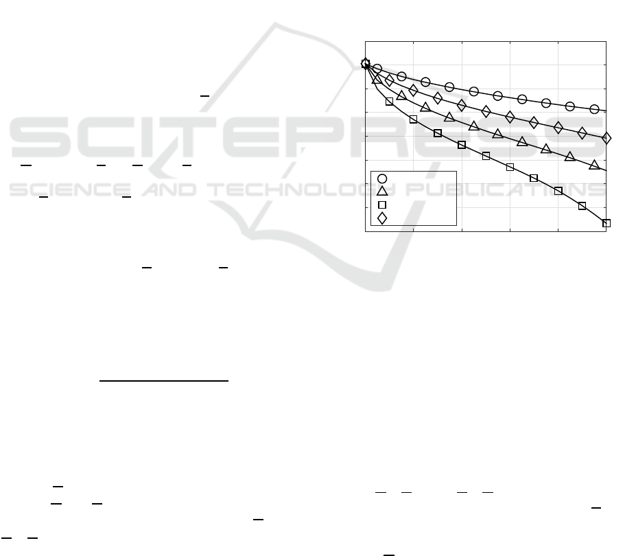
A(z). Fig. 1 shows the normalized remaining

off-diagonal energy η

(i)

versus iteration index i for

each PEVD algorithm. Obviously, both the SMD and

MSME-SMD algorithms outperform SBR2 and MS-

SBR2 in terms of eliminating the off-diagonalenergy.

This is due to the fact that a full EVD operation is

applied in SMD algorithm family at each iteration,

which can transform more off-diagonal elements onto

diagonal. However, this is also one of the factors

which causes the SMD algorithm family much higher

computational cost than the SBR2 algorithm. Obvi-

ously the MS-SBR2 algorithm requires much fewer

iterations than the conventional SBR2 algorithm to

achieve the same level of diagonalization. However,

it should also be noticed that each iteration within

MS-SBR2 involves more rotation steps, which means

the computational costs between them are compara-

ble. Nonetheless, the MS-SBR2 algorithm has been

found to converge faster than SBR2 especially when

decomposing high dimension para-Hermitian polyno-

mial matrices. For further details of the algorithm,

including numerical examples and proof of conver-

gence, see (Wang et al., 2015).

0 20 40 60 80 100

-16

-14

-12

-10

-8

-6

-4

-2

iteration index i →

5 · l og

E{η

(i)

} (indB) →

SBR2

SMD

MSME-SMD

MS-SBR2

Figure 1: Comparisons of normalized off-diagonal energy

among different PEVD algorithms, showing ensemble av-

erages versus iterations.

As shown by the simulation results, the off-

diagonal energy with the use of the investigated

PEVD algorithms becomes neglectable small at a suf-

ﬁciently high number of iterations.

4.5 Accuracy of the Decomposition

There are two main factors which can affect the accu-

racy of the decomposition. Firstly, since the decom-

position is performed upon the two para-Hermitian

matrices C

(z)

C(z) and

C(z)C(z) as shown in equa-

tions (5) and (6), the resulting diagonal matrix Σ

Σ(z)

might be less accurate than that found by the way of

operating the decomposition directly upon the chan-

nel matrix C

(z).

Secondly, for the broadband MIMO application,

OPTICS 2016 - International Conference on Optical Communication Systems

a strictly diagonalized channel matrix is required.

However, the proposed PMSVD method can only

generate an approximately diagonal matrix subject to

the pre-speciﬁed stop condition of the algorithm, so

there will be errors when assuming all off-diagonal

elements of the matrix Σ

(z) are equal to zero. In ad-

dition, due to the fact that the orders of the polyno-

mial matrices increase as the iteration goes through-

out the PEVD process, proper truncations are usually

required for the matrices U

(z), Σ

Σ(z), and V(z) in or-

der to keep orders as small as possible and reduce the

computational cost of the algorithm. This can cause

a very small proportion of the total Frobenius norm

of the matrix being eliminated, which also can bring

errors.

5 OPTICAL MIMO TESTBED

An optical MIMO system can be formed by feeding

different sources of light into the ﬁbre, which can ac-

tivate different optical mode groups. This can be car-

ried out by using centric and eccentric light launching

conditions and subsequent combining of the activated

different mode groups with a fusion coupler as shown

in Fig. 2 (Sandmann et al., 2014).

(low order mode path)

(high order mode path)

Figure 2: Transmitter side fusion coupler for launching dif-

ferent sources of light into the MMF.

Different sources of light lead to different power

distribution patterns at the ﬁbre end depending on the

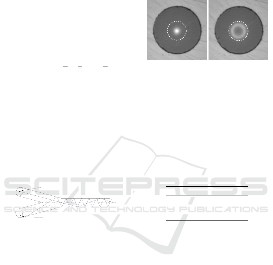
transmitter side light launch conditions. Fig. 3 high-

lights the measured mean power distribution pattern

at the end of a 1.4 km multi-mode ﬁbre (MMF). Here,

for splitting the different mode groups a similar fusion

coupler is used.

The measurement setup depicted in Fig. 4 shows

the testbed with the utilized devices for measuring

the system properties of the optical MIMO channel

in form of its speciﬁc impulse responses needed for

modelling the MIMO data transmission.

A picosecond laser unit is chosen for generating

the 25 ps input pulse. This input pulse is used to mea-

sure separately the different SISO channels within the

MIMO system. Since the used picosecond laser unit

doesn’t guarantee a fully ﬂat frequency spectrum in

the region of interest, the captured signals have to be

deconvolved (Sandmann et al., 2013). The obtained

impulse responses are forming the base for modelling

Figure 3: Measured mean power distribution pattern when

using the fusion coupler at the transmitter side (left: cen-

tric mode excitation; right: eccentric mode excitation); the

dotted line represents the 50 µm core size.

the MIMO transmission system. Fig. 5 highlights the

resulting electrical MIMO system model.

6 SIMULATION RESULTS

In this work, the BER quality is studied by using ﬁxed

transmission modes with a spectral efﬁciency of 8

bit/s/Hz. The analyzed quadrature amplitude modu-

lation (QAM) constellations, equivalent to how many

bits are allocated to each layer, are shown in Tab. 1.

Table 1: Transmission Modes.

throughput layer 1 layer 2

8 bit/s/Hz 256 0

8 bit/s/Hz 64 4

8 bit/s/Hz 16 16

The channel, studied in this contribution, is a mea-

sured (2× 2) optical MIMO channel.

Here, the measurement results within a 1.4 km

(2× 2) optical MIMO channel at an operating wave-

length of 1576 nm, depicted in Fig. 6, have been used

(Sandmann et al., 2015b). The graphs clearly show

the effect of chromatic dispersion being characteristic

at this operating wavelength in a standard ﬁber.

Applying PMSVD to this frequency-selective

MIMO channel results in layers having a time-

dispersive characteristic and hence ISI occurs on each

layer. The ISI is removed by applying a T-spaced zero

forcing (ZF) equalizer and therefore this equalization

scheme is entitled T-PMSVD. The equalizers mod-

ify the noise power on each layer differently, which

is expressed by the weighting factors θ

ℓ

, with ℓ de-

noting the layer index. These factors determine the

layer speciﬁc SNRs and hence also the total BER per-

formance (Sandmann et al., 2015c). Calculating the

PMSVD of the optical MIMO channel using differ-

ent PEVD algorithms shows that the weighting fac-

tors θ

ℓ

listed in Tab. 2 are identical. This implies

Polynomial Matrix SVD Algorithms for Broadband Optical MIMO Systems

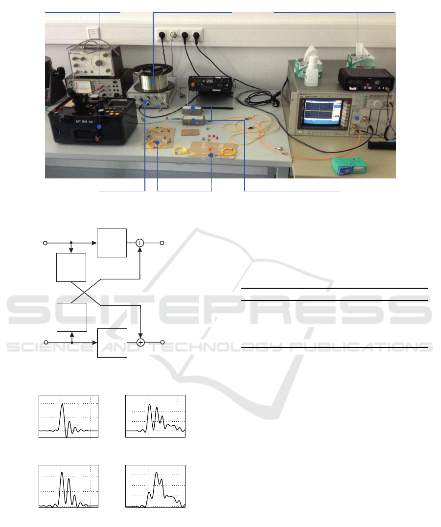
Light Launching Unit (splicer) 1.4 km multi-mode fibre channel Sampling Oscilloscope with MSM Photo Detector

Picosecond Laser Laser-diode ( ≈ 1.3 μm or 1.55 µm)Fusion Couplers

Figure 4: Measurement setup for determining the MIMO speciﬁc impulse responses.

s 1

(t)

s 2

(t)

k 1

(t)

k 2

(t)

Figure 5: Electrical (2× 2) MIMO system model (example:

= n

= 2).

2 4

0.0

0.5

1.0

2 4

0.1

0.2

0.3

2 4

0.1

0.2

2 4

0.05

0.1

0.15

t (inns) →t (inns) →

1 1

(t) →

1 2

(t) →

2 1

(t) →

2 2

(t) →

Figure 6: Measured electrical MIMO impulse responses

with respect to the pulse frequency f

= 1/T

= 620 MHz

at 1576 nm operating wavelength.

that the achievable BER is independent of the ap-

plied PEVD algorithms for the studied (2× 2) MIMO

channel. In addition, the remaining off-diagonal en-

ergy ε =

∑

kC(τ)k

−

∑

kΣ

Σ(τ)k

is negligibly small,

Table 2: Comparisons of remaining off-diagonal energy ε

and noise ampliﬁcation factor θ

ℓ

among different PEVD

algorithms, showing that different PEVD algorithms can

achieve exactly the same BER performance subject to the

same stop criterion of the PEVD algorithms, i.e. the thresh-

old of the off-diagonal element ε = 10

−4

algorithms ε θ

SBR2 1.26× 10

−6

37.22 4243.46

SMD 1.26× 10

−6

37.22 4243.46

MSME-SMD 1.26×10

−6

37.22 4243.46

MS-SBR2 1.26× 10

−6

37.22 4243.46

which means that the CI has been signiﬁcantly elimi-

nated.

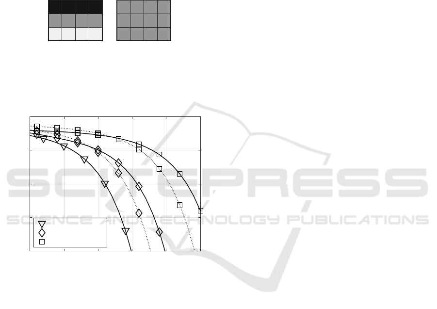
The BER performance results, obtained by apply-

ing the SBR2 algorithm for calculating the PMSVD,

are depicted in Fig. 8 for the different QAM constel-

lation sizes. The (256, 0) transmission scheme shows

the best performance results suggesting that not all

layers should be activated when optimizing the BER

performance.

Based on the unequal weighting of the layers, PA

can be used to balance the bit-error probabilities in

the different numbers of activated MIMO layers. Re-

garding the channel quality, the BER performance is

affected by the layer-speciﬁc weighting factors, the

chosen QAM-constellation size as well as the layer-

speciﬁc noise power. Since optimal PA solutions

are notably computationally complex to implement,

a suboptimal solution which concentrates on the ar-

gument of the complementary error function is inves-

tigated in this work (Ahrens et al., 2015).

By applying T-PMSVD the ISI is fully removed

by the equalizer and thus for each layer the half ver-

tical eye opening of the receive signal equals the

OPTICS 2016 - International Conference on Optical Communication Systems

half-level amplitude of the transmitted symbols. The

drawback of the T-PMSVD is that the noise and hence

the noise power is weighted differently on each layer

by the equalizer coefﬁcients expressed by the factors

and θ

as shown in Tab. 2. The proposed PA al-

gorithm distributes the available transmit power such

that the layer speciﬁc SNRs are equal (Sandmann

et al., 2015c; Ahrens et al., 2015). The resulting SNRs

for the proposed PA scheme in T-PMSVD systems are

visualized in Fig. 7.

layer ℓ

time k

layer ℓ

time k

Figure 7: Illustration of the remaining SNRs in T-PMSVD

systems without applying PA (left) and with layer-based PA

(right). The color black refers to high and white to low SNR

values.

35 40 45 50 55 60

-8

-6

-4

-2

BER

→

10 · log

) (indB) →

(256,0) QAM

(64,4) QAM

(16,16) QAM

Figure 8: BER with PA (dotted line) and without PA

(solid line) by applying the T-PMSVD equalization scheme,

showing the comparisons among different transmission

modes when transmitting over the optical (2 × 2) MIMO

channel.

7 CONCLUSION

We have investigated the PMSVD technique in the

application of decomposing the channel matrix of a

measured (2×2) optical MIMO system, and different

iterative PEVD algorithms have been utilized for the

calculation of PMSVD. Despite the different number

of iterations needed to minimize the off-diagonal ele-

ment below a given threshold, all investigated PEVD

algorithms show the same BER performance.

ACKNOWLEDGEMENTS

This work has been funded by the German Ministry

of Education and Research (No. 03FH016PX3).

REFERENCES

Ahrens, A., Sandmann, A., Lochmann, S., and Wang, Z.

(2015). Decomposition of Optical MIMO Systems us-

ing Polynomial Matrix Factorization. In 2nd IET In-

ternational Conference on Intelligent Signal Process-

ing (ISP), London (United Kingdom).

Corr, J., Thompson, K., Weiss, S., McWhirter, J. G., Redif,

S., and Proudler, I. K. (2014). Multiple Shift Maxi-

mum Element Sequential Matrix Diagonalisation for

Parahermitian Matrices. In IEEE SSP Workshop,

pages 312–315, Gold Coast (Australia).

Haykin, S. S. (2002). Adaptive Filter Theory. Prentice Hall,

New Jersey.

Kühn, V. (2006). Wireless Communications over MIMO

Channels – Applications to CDMA and Multiple An-

tenna Systems. Wiley, Chichester.

McWhirter, J. G. and Baxter, P. D. (2004). A Novel Tech-

nique for Broadband Singular Value Decomposition.

In 12th Annual ASAP Workshop, MA (USA).

McWhirter, J. G., Baxter, P. D., Cooper, T., Redif, S.,

and Foster, J. (2007). An EVD Algorithm for Para-

Hermitian Polynomial Matrices. IEEE Trans. SP,

55(5):2158–2169.

Raleigh, G. G. and Ciofﬁ, J. M. (1998). Spatio-Temporal

Coding for Wireless Communication. IEEE Transac-

tions on Communications, 46(3):357–366.

Raleigh, G. G. and Jones, V. K. (1999). Multivariate

Modulation and Coding for Wireless Communication.

IEEE Journal on Selected Areas in Communications,

17(5):851–866.

Redif, S., Weiss, S., and McWhirter, J. G. (2015). Sequen-

tial Matrix Diagonalization Algorithms for Polyno-

mial EVD of Parahermitian Matrices. IEEE Trans. SP,

61(1):81–89.

Sandmann, A., Ahrens, A., and Lochmann, S. (2013).

Signal Deconvolution of Measured Optical MIMO-

Channels. In XV International PhD Workshop OWD,

pages 278–283, Wisla, Poland.

Sandmann, A., Ahrens, A., and Lochmann, S. (2014). Ex-

perimental Description of Multimode MIMO Chan-

nels utilizing Optical Couplers. In ITG-Fachbericht

248: Photonische Netze, pages 125–130, Leipzig

(Germany). VDE VERLAG GmbH.

Sandmann, A., Ahrens, A., and Lochmann, S. (2015a).

Modulation-Mode and Power Assignment in SVD-

Assisted Broadband MIMO Systems using Polyno-

mial Matrix Factorization. Przeglad Elektrotech-

niczny, 04/2015:10–13.

Sandmann, A., Ahrens, A., and Lochmann, S. (2015b). Per-

formance Analysis of Polynomial Matrix SVD-based

Polynomial Matrix SVD Algorithms for Broadband Optical MIMO Systems

Broadband MIMO Systems. In Sensor Signal Pro-

cessing for Defence Conference (SSPD), Edinburgh

(United Kingdom).

Sandmann, A., Ahrens, A., and Lochmann, S. (2015c).

Resource Allocation in SVD-Assisted Optical MIMO

Systems using Polynomial Matrix Factorization. In

ITG-Fachbericht 257: Photonische Netze, pages 128–

134, Leipzig (Germany). VDE VERLAG GmbH.

Sandmann, A., Ahrens, A., and Lochmann, S. (2016). Ex-

perimental Evaluation of a (4x4) Multi-Mode MIMO

System Utilizing Customized Optical Fusion Cou-

plers. In ITG-Fachbericht 249: Photonische Netze,

pages 101–105, Leipzig (Germany). VDE VERLAG

GmbH.

Singer, A. C., Shanbhag, N. R., and Bae, H.-M. (2008).

Electronic Dispersion Compensation– An Overwiew

of Optical Communications Systems. IEEE Signal

Processing Magazine, 25(6):110–130.

Ta, C. and Weiss, S. (2007). A Design of Precoding

and Equalisation for Broadband MIMO Systems. In

Asilomar Conf. Signals, Systems & Computers, pages

1616–1620, Paciﬁc Grove, (CA).

Tse, D. and Viswanath, P. (2005). Fundamentals of Wireless

Communication. Cambridge, New York.

Vaidyanathan, P. P. (1993). Multirate Systems and Filter

Banks. Prentice Hall, New Jersey.

Wang, Z., McWhirter, J. G., Corr, J., and Weiss, S. (2015).

Multiple Shift Second Order Sequential Best Rotation

Algorithm for Polynomial Matrix EVD. In 23rd EU-

SIPCO, pages 849–853, Nice (France).

Wang, Z., Sandmann, A., McWhirter, J., and Ahrens, A.

(2016). Multiple Shift SBR2 Algorithm for Calculat-

ing the SVD of Broadband Optical MIMO Systems.

In 39th International Conference on Telecommunica-

tions and Signal Processing (TSP), Vienna (Austria).

Winzer, P. J. and Foschini, G. J. (2011). MIMO Ca-

pacities and Outage Probabilities in Spatially Multi-

plexed Optical Transport Systems. Optics Express,

17(19):16680–16696.

OPTICS 2016 - International Conference on Optical Communication Systems