
The Sourcing Problem
Energy Optimization of a Multisource Elevator
Chlo
´
e Desdouits
1,2,3
, Mazen Alamir
2
, Rodolphe Giroudeau
3
and Claude Le Pape
1
1
Strategy Technology, Schneider Electric Industries SAS,
38 TEC, 37 quai Paul-Louis Merlin, 38050 Grenoble Cedex 09, France
2
Control Systems Department, GIPSA-lab,
UMR 5216 CNRS - Grenoble INP - Universit
´
e Joseph Fourier - Universit
´
e Stendhal,
11 rue des Math
´
ematiques - Grenoble Campus - BP46, 38402 Saint Martin d’H
`
eres Cedex, France
3
Computer Science Department, LIRMM,
UMR 5506 - Universit
´
e Montpellier 2, CC477,
161 rue Ada, 34095 Montpellier Cedex 5, France
Keywords:
Energy Optimization, Control of Dynamic Systems, Linear Programming, Rule-based Algorithms.
Abstract:
As the interest in regulating energy usage and in the demand-response market is growing, new energy man-
agement algorithms emerge. In this paper, we propose a formalization of “the sourcing problem” and its
application to a multisource elevator. We propose a linear formulation that, coupled with a low level rule-
based controller, can solve this problem. We show in the experiments that a compromise between reducing
consumption peaks and minimizing the energy bill has to be reached.
1 INTRODUCTION
Reducing energy consumption is a major issue nowa-
days; not only in order to restrain the ecological im-
pact on the planet, but also to both respect building
norms and minimize industrial and residential activ-
ities’ energy bill. In order to achieve this goal, one
can act on energy consumption by optimizing the
amount of energy consumed, or by shifting consump-
tion during the day. But one can also control one’s
energy consumption impact, by adding renewable en-
ergy sources and storage units. Thus, an “energy hub”
is created.
If one chooses this second possibility, a new op-
timization problem arises. The energy hub has to de-
cide which energy source to be used at which mo-
ment. We call this problem “the sourcing problem”
and formalize it in Section 2.
In this paper, we solve the sourcing problem for a
multisource elevator, as the newest generations of el-
evators are equipped with energy storage to ensure a
minimum autonomy in case of power failure. This is
crucial for safety (e.g. to evacuate people with re-
duced mobility) and energy storage may also offer
flexibility in power management. In Section 3, the
reader is given an glimpse of what can be done for
dealing with energy sourcing issues of those multi-
source elevators.
Section 4 gives details on our solution to solve the
sourcing problem. First by describing interactions be-
tween our two coupled controllers. Then by explain-
ing the linear formulation used to compute a sourcing
strategy. And finally by giving some details on how
our low-level rule-based controller takes strategy into
account.
Afterwards, experiments are conducted in Sec-
tion 5 to highlight advantages and drawbacks of that
method, as well as parameters influencing its achieve-
ments.
Finally, Section 6 concludes the paper and intro-
duces future work.
2 THE SOURCING PROBLEM
We call “prosumers”, entities that consume and/or
produce energy. An energy hub allows each prosumer
to consume power produced by all other prosumers at
the same time.
Definition 1. Let P be a set of n
p
prosumers, all con-
nected to the same energy hub h.
Desdouits, C., Alamir, M., Giroudeau, R. and Pape, C.
The Sourcing Problem - Energy Optimization of a Multisource Elevator.
DOI: 10.5220/0005947600190030
In Proceedings of the 13th International Conference on Informatics in Control, Automation and Robotics (ICINCO 2016) - Volume 1, pages 19-30
ISBN: 978-989-758-198-4
Copyright
c
2016 by SCITEPRESS – Science and Technology Publications, Lda. All rights reserved
19

We differentiate three kinds of prosumers: the set
S of storage units, the set P of controllable producers
and the set E of the others. Thus, these sets form a
partition of the whole set of prosumers.
Definition 2. Let S = {π
S
1
, . . . , π
S
n
S
} be the set of stor-
age units, P = {π
P
1
, . . . , π
P
n
P
} be the set of controllable
producers or consumers, and E = {π
E
1
, . . . , π
E
n
E
} be
the set of the other prosumers. Then, P = S ∪ P ∪ E.
Each prosumer can consume and/or produce
power, depending on its physical capabilities.
Definition 3. For a given prosumer π
i
∈ P , let p
min
i
≤
0 (resp. p
max
i
≥ 0) be the minimum (resp. maximum)
instantaneous power of π
i
. Then, at a given time t, let
p
min
i
≤ p
i
[t] ≤ p
max
i
be the instantaneous power pro-
duced by π
i
if p
i
[t] is positive, or consumed by π
i
if
p
i
[t] is negative
1
.
A system composed of an energy hub and its pro-
sumers can be represented by a star oriented graph.
Definition 4. Let G = (P ∪ h,A) be a star oriented
graph rooted in h where P ∪ h are the nodes of the
graph and A are the weighted arcs. There is an arc
(π
i
, h) if p
max
i
> 0 and the weight of the arc is p
max
i
.
In the same way, there is an arc (h,π
i
) if p
min
i
< 0 and
the weight of the arc is p
min
i
.
We suppose that time can be sampled in a regular,
uniform way.
Definition 5. Let τ ∈ R be the sampling period (ex-
pressed in hours), and H ∈ N be the number of peri-
ods considered. Then time-steps are expressed in the
following way: t
l
= t
l−1
+ τ = l × τ, ∀l ∈ {0, . . . , H}.
Finally, each controllable producer has an energy
cost function that gives the price associated to an en-
ergy consumption or production of this prosumer.
Definition 6. ∀π
i
∈ P, let cost
π
i
: [p
min
i
, p
max
i
] → R be
the energy cost function associated to π
i
.
Then, we can define sourcing problems:
Instance: a set of prosumers P = P ∪ S ∪ E,
a graph G = (P ∪ h, A),
a period τ ∈ R,
a time horizon H ∈ N,
a set of cost functions:
{cost
i
, ∀π
P
i
∈ P}
Solution: S, a n
p
× H matrix of p
i
[t]
1
Power is expressed in Watts and energy in Watt hours.
Quest. 1: given p
max
hub
∈ R the allowed residual
power of the energy hub, does a ma-
trix S exist such that:
∀l ∈ {0, . . . , H −1},
− p
max
hub
≤
n
p
∑
i=1
p
i
[t
l
] ≤ p
max
hub
(1)
Can the energy hub be autonomous?
Quest. 2: given p
max
P
∈ R the allowed power
peak of controllable producers, does
a matrix S exist such that:
∀l ∈ {0, . . . , H −1},
max
π
i
∈P
p
i
[t
l
] ≤ p
max
P
(2)
Can power peaks purchased from
controllable producers stay below a
given value?
Quest. 3: given cost
max
hub
∈ R the allowed energy
bill, does a matrix S exist such that:
H−1
∑
l=0
∑
π
i
∈P
cost
π
i
(p
i
[t
l
] × τ)
≤ cost
max
hub
(3)
Can the energy bill stay below a
given value?
These three objectives are sometimes antagonis-
tic.
In this paper, we consider the following applica-
tion of the sourcing problem. The set P of prosumers
is composed of: an elevator π
1
, that can get energy
from a battery π
2
, a supercapacitor π
3
, the grid π
4
and
Energy
hub
Elevator
π
1
Solar
panels
π
5
Grid
π
4
Battery
π
2
Supercapacitor
π
3
Dissipation
resistor
π
6
p
min
1
p
max
1
p
max
4
p
max
5
p
min
2
p
max
2
p
min
3
p
max
3
p
min
6
Figure 1: The elevator sourcing problem.
ICINCO 2016 - 13th International Conference on Informatics in Control, Automation and Robotics
20

a solar panel π
5
. The supercapacitor is here to absorb
power peaks above the maximum power capability of
the battery. But the former is more expensive than the
latter. Moreover, energy can be recovered from the
elevator when the brakes are applied. Finally, energy
can be dissipated in a resistor π
6
if there is too much.
The partition of P is the following: E = {π
1
, π
5
},
P = {π
4
, π
6
}, S = {π
2
, π
3
}. An illustration of the ele-
vator sourcing problem is given in Figure 1.
As it is a real-life application, the three objectives
corresponding to questions above have to be achieved
simultaneously. The goal is to minimize power peaks
purchased from the grid and the energy bill while en-
suring that the hub is autonomous.
3 STATE OF THE ART
Energy optimization systems have been widely stud-
ied in the literature, especially in the past few years.
In the following state of the art, we present research
works dedicated to energy sourcing of multisource el-
evators.
A very comprehensive work on energy systems
for elevators is proposed by (Paire et al., 2010).
They have designed a physical multi-source system
to power an elevator. In the paper, rules are used to
charge or discharge batteries depending on whether
the electrical current is below or above a given refer-
ence. This control method may be reduced to a simple
“if, then, else” structure achieved by physical compo-
nents.
Likewise, (Tominaga et al., 2002) presents three
rule-based methods to control a battery coupled with
an elevator. This method takes into account peak/off-
peak tariffs and reduces energy consumption cost by
storing energy recovered from the elevator.
These methods allow controlling very reactively
the system, but cannot take into account optimally ex-
ternal considerations such as the electricity tariff or
battery state of health. Therefore, these control meth-
ods may not be efficient regarding economical objec-
tives.
On the other hand, (Bilbao and Barrade, 2012)
have proposed a General Energy and Statistical De-
scription (GESD) of the possible missions of an ele-
vator and an energy manager based on dynamic pro-
gramming. Their energy manager is inspired by stock
management theory and minimizes the sum of en-
ergy (i) absorbed from the grid, (ii) dissipated in the
braking resistor and (iii) not provided to the elevator.
The optimization is done off-line. This method de-
duces economically optimal solutions from consump-
tion probabilities. But elevator usage is unpredictable
by nature and there is no given alternative when the
strategy is not applicable.
Finally, in (Sachs, 2005), authors summarize dif-
ferent ways to optimize choices of elevator physical
components (motor, drive, etc). An appropriate sizing
of these components is a way to optimize energy con-
sumption but it should be coupled with a good control
algorithm of multiple sources of energy.
From these observations, we have decided to pro-
pose a two-layer optimization that can achieve reac-
tive control of low-level equipment as well as com-
pute economically optimal sourcing strategy. As part
of the European Arrowhead project, we published a
first description of a linear program to solve the mul-
tisource elevator problem in (Desdouits et al., 2015).
We also described, in (Boutin et al., 2014), the inter-
actions between our control method and partner com-
ponents. In the current paper, we formalize the sourc-
ing problem, improve our linear formulation and give
details on Local Controllers. More accurate experi-
mental results than before are additionally given.
4 PROPOSED SOLUTION
In this section, we give a centralized rule-based algo-
rithm for the energy hub controller, but we also could
overlay another controller already implemented. We
call these controllers “Local Controllers”, and we ab-
breviate LC. They have to be embedded and highly
reactive, thus they cannot compute the best sourcing
strategy on a long time-frame. Therefore, we decided
to compute a sourcing strategy with a “Strategic Op-
timizer” (abbreviated SO), and to send next strategic
instructions to LC regularly.
Definition 7. Let us call the plan computed by SO a
strategy, and the set-point computed by LC a tactic.
Hereafter, we start by presenting data that feed
components and interactions between them.
4.1 Data and Interactions
In this sub-section, we first describe how we draw
samples of elevator usage. Then we explain how we
compute forecasts used by SO. Finally, we show com-
ponents interactions and their dynamic.
4.1.1 Elevator Usage Description
The building considered is a business tower with nine
floors and the elevator has the following characteris-
tics: standby consumption: 50 W, cabin mass: 750
kg, counterweight mass: 850 kg, nominal velocity:
1.0 ms
−1
.
The Sourcing Problem - Energy Optimization of a Multisource Elevator
21

We simulate user calls to the elevator with a statis-
tical model. This model distinguishes multiple types
of travels: morning and afternoon arrivals and depar-
tures, lunch breaks, inter-floor travels, arrivals and de-
partures of external visitors. Statistical laws are iden-
tified based on historical data. For each travel type
and relevant pair of floors, these laws provide infor-
mation on the number of people moving during the
day (depending on day-of-week, week-of-year, etc.),
the distribution of their weights, the distribution of the
times of the people movements during the day, and the
probability that two similar movements are grouped
(e.g., several people going to lunch together). A ran-
dom generator is used on this basis to generate sce-
narios.
Moreover, we have implemented a tactic to an-
swer user calls to the elevator. That tactic considers
calls in chronological order to choose the destination
of the elevator. But, it stops the elevator along the way
if another call destination is on this way. That seems
to be the tactic implemented in the biggest part of the
elevators.
On the other hand, we have an energy model of
the elevator that allows us to compute energy con-
sumption regarding the chosen travel and the weight
of passengers. The data used in this model include
the weight of the cabin and counterweight, the length
and weight of the cable, the elevator’s base power and
nominal speed, the altitude of the departure and ar-
rival floors, and efficiency for both energy-consuming
and energy-producing travels.
4.1.2 Forecasts
SO is fed by a forecast f, that is a |P ∪ E| × H ma-
trix, with H the number of periods considered by SO.
For prosumers in P, the tariff is forecasted, while for
prosumers in E, the produced and consumed quantity
is forecasted. In this paper, forecasts are considered
exact (issues concerning robustness to forecasts un-
certainties will be considered in a future paper).
In our use case, a forecast is composed of: (i) the
predicted amount of energy consumed / produced by
the elevator, (ii) the predicted solar production, (iii)
the predicted grid energy tariff. Dissipation is as-
sumed to have no cost.
The ideal solar production prediction uses pre-
dicted irradiance data of a typical sunny day. We con-
sider that 2 square meters of solar panels are installed
on the roof top of the building, and are dedicated to
the elevator. These solar panels are supposed well ori-
ented towards the sun and having a yield of 15%.
The electricity tariff considered in the experiments
is a typical peak / off-peak French tariff: 0.00015 /
0.00010 e/Wh.
Regarding the elevator, we use data described in
sub-section 4.1.1 to simulate several daily scenarios
and compute the average energy production or con-
sumption for each SO period. An alternative could
be to use standard machine learning techniques to di-
rectly forecast energy production or consumption for
each SO period.
4.1.3 Interactions and Dynamic
LC has to be highly reactive. For the multisource el-
evator application, we estimate a relevant time-step
is one second, iterated every seconds. On the other
hand, SO has to consider sufficiently long time-steps
to get relevant forecasts, and a sufficiently long hori-
zon to take into account energy price variations. Thus,
a fifteen minutes period with a 24h horizon is relevant
for the multisource elevator, and the problem is re-
solved every hours. The dynamic of interactions is
illustrated on Figure 2.
In a real product, LC would probably be embed-
ded into the energy hub. While SO could be proposed
as a web service. We can see on the figure that LC
and SO are separated components that communicate
only through a strategic instruction. An instruction is
composed of a target time, and an array of n
p
cells:
one per prosumer connected to the energy hub. For
storage units, an instruction is expressed as a target
state of charge. For controllable producers, an in-
struction is expressed as mean power. For the other
prosumers (that are supposed non controllable), in-
structions are empty. An instruction can be sent over
a network or shared by components running into the
same computer. That allows flexible business models.
Moreover, SO needs to know the current state of
charge of every storage units and the current availabil-
ity of controllable producers.
Finally, LC applies the computed tactic that is a
vector of n
p
power values, on the multisource system.
LC is fed with solar radiation, electricity tariff and
users’ calls to the elevator.
Runs every hour
Runs every second
Strategic
Optimizer
Local
Controller
Multisource
system
strategy for the
next hour
Power set-point
for all prosumers
Current state
and flexibilities
Current
state
forecast f (15 mn
timestep, 24 h horizon)
Figure 2: Software components interactions.
ICINCO 2016 - 13th International Conference on Informatics in Control, Automation and Robotics
22

4.2 Strategic Optimizer
The problem solved by SO consists of finding the best
sources of energy to be used, factoring in the storage
capacities, during a long time frame. The goal is to
minimize costs related to energy purchasing and bat-
tery usage within the time frame, while ensuring the
hub is autonomous.
4.2.1 A Generic Formulation Depending on
Prosumers Kind
Let us suppose that the optimization period is a con-
stant τ, and that the number of periods in the opti-
mization horizon is denoted H.
Definition 8. Let e
i
[t] = p
i
[t] × τ be the energy
amount produced by prosumer π
i
over a period τ.
Thereafter decision and state variables are defined,
depending on prosumers kind:
• Storage units: ∀π
i
∈ S,
– ∀l ∈ {0, . . . , H − 1}, 0 ≤ e
ch
i
[t
l
] ≤ −p
min
i
× τ
(resp. 0 ≤ e
dis
i
[t
l
] ≤ p
max
i
× τ) the amount of
energy charged into (resp. discharged from)
the prosumer π
i
(that is a storage unit) between
time t
l
and time t
l+1
= t
l
+ τ. Thus e
i
[t
l
] =
e
dis
i
[t
l
] − e
ch
i
[t
l
].
– ∀l ∈ {0, . . . , H}, 0 ≤ x
i
[t
l
] ≤ 1 the state of charge
of the prosumer π
i
at time t
l
.
• Controllable producers: ∀π
i
∈ P,
– ∀l ∈ {0, . . . , H − 1}, 0 ≤ e
purch
i
[t
l
] ≤ p
max
i
× τ
(resp. 0 ≤ e
sold
i
[t
l
] ≤ −p
min
i
× τ) the amount
of energy purchased from (resp. sold to) the
prosumer π
i
(that is a controllable producer)
between time t
l
and time t
l+1
= t
l
+ τ. Thus
e
i
[t
l
] = e
purch
i
[t
l
] − e
sold
i
[t
l
].
• Non-controllable prosumers: ∀π
i
∈ E,
– ∀l ∈ {0, . . . , H − 1}, p
min
i
× τ ≤ e
i
[t
l
] = f
i
[t
l
] ≤
p
max
i
× τ the forecasted production (if positive)
or consumption (if negative) of the prosumer π
i
between time t
l
and time t
l+1
= t
l
+ τ. These
e
i
are not decision variables but constant data
given by an external forecast.
Remark: Although storage units charge and dis-
charge could be modeled as a single variable e
i
, two
variables (e
ch
i
and e
dis
i
) are used in our model, be-
cause there are two different yields that impact the
charge and the discharge. However, we do not want
to charge and discharge the same storage unit at the
same time, thus both variables are minimized in the
objective function.
Lemma 4.1. In all optimal solutions,
∀l ∈ {0, . . . , H −1}, ∀π
i
∈ S, e
ch
i
[t
l
] = 0 ∨ e
dis
i
[t
l
] = 0.
Proof. Assume
ˆ
e, an optimal solution, such that there
exists 0 ≤ l ≤ H −1 where both ˆe
ch
i
[t
l
] and ˆe
dis
i
[t
l
] are
strictly positive. Then, let us consider another so-
lution e
0
where all decision variables have the same
value except that:
e
ch
0
i
[t
l
] = ˆe
ch
i
[t
l
] − min( ˆe
ch
i
[t
l
], ˆe
dis
i
[t
l
])
e
dis
0
i
[t
l
] = ˆe
dis
i
[t
l
] − min( ˆe
ch
i
[t
l
], ˆe
dis
i
[t
l
])
As e
ch
0
i
[t
l
] and e
dis
0
i
[t
l
] are both penalized in the objec-
tive function, then solution e
0
admits a lower cost than
solution
ˆ
e that was optimal by assumption.
The following constraints must be taken into account:
• A minimum energy amount must be kept into stor-
age units.
∀π
i
∈ S, ∀l ∈ {0, . . . , H},
x
i
[t
l
] + ρ
minSOC
i
[t
l
] ≥ c
minSOC
i
, (4)
For this constraint, a new slack variable is defined:
0 ≤ ρ
minSOC
i
[t
l
] ≤ c
minSOC
i
is the percentage of stor-
age unit state of charge under a given minimum
value c
minSOC
i
at time t
l
. Then, c
minSOC
i
is the ratio
of the storage unit state of charge that the energy
hub needs to ensure security in case of grid fail-
ure. The ρ
minSOC
i
variables must be null except in
the case of grid failure, so they are penalized in
the objective function (cf Equation (9) ).
• The energy-related equation of the energy hub
must be satisfied: the sum of consumed and pro-
duced energy between time t
l
and time t
l+1
= t
l
+τ
must be equal.
∀l ∈ {0, . . . , H − 1},
∑
i∈P
(e
i
[t
l
]) = 0 (5)
• The state of charge of storage units must be up-
dated at each time-step with the energy charged
and discharged.
∀π
i
∈ S, ∀l ∈ {0, . . . H −1},
x
i
[t
l+1
] = x
i
[t
l
] +
c
cy
i
c
ce
i
× e
ch
i
[t
l
]
−
1
c
dy
i
× c
ce
i
× e
dis
i
[t
l
] (6)
where c
ce
i
is the energy capacity of the storage unit
and c
cy
i
(resp. c
dy
i
) is the charging (resp. discharg-
ing) yield of the storage unit. Yields are normal-
ized between 0 and 1.
The Sourcing Problem - Energy Optimization of a Multisource Elevator
23

• Let a new slack variable ∀l ∈ {0, . . . H − 1}, 0 ≤
ρ
stab
i
[t
l
] ≤ p
max
i
− p
min
i
be the difference between
the amount of energy purchased from a control-
lable producer π
i
at time t
l
and the amount of en-
ergy purchased from the same controllable pro-
ducer at time t
l−1
. This value has to be penal-
ized in the objective function. The associated con-
straints are:
∀π
i
∈ P,∀l ∈ {0, . . . H −1},
e
i
[t
l−1
] − e
i
[t
l
] − ρ
stab
i
[t
l
] ≤ 0 (7)
e
i
[t
l
] − e
i
[t
l−1
] − ρ
stab
i
[t
l
] ≤ 0 (8)
Please note that, for the first period, e
i
[t
l−1
] is set
to the instruction computed for prosumer π
i
dur-
ing SO last run. If the current execution is the first
one, e
i
[t
l−1
] is set to zero.
• Depending on the exact use case, cyclical con-
straints (or additional cost factors), such as requir-
ing the battery to be full at the beginning of the
morning can be added.
Given those constraints, our economical objective
function is given by Equation (9).
Minimize
H−1
∑
l=0
"
∑
π
i
∈P
−c
sold
i
[t
l
] × e
sold
i
[t
l
] + c
purch
i
[t
l
] × e
purch
i
[t
l
]
+ min
"
min
π
j
∈P
(c
purch
j
[t
l
])
10
,
min
π
j
∈S
(c
aging
j
)
2
#
× ρ
stab
i
[t
l
]
!
+
∑
π
i
∈S
c
aging
i
2
× e
ch
i
[t
l
] +
c
aging
i
2
× e
dis
i
[t
l
]
+ 2 × max
π
j
∈P
(c
purch
j
[t
l
]) × ρ
minSOC
i
[t
l
]
!#
(9)
where c
purch
i
[t
l
] is the electricity buying price at time
t
l
and c
sold
i
[t
l
] is the electricity selling price at time t
l
thus −c
sold
i
[t
l
] × e
sold
i
[t
l
] + c
purch
i
[t
l
] × e
purch
i
[t
l
] is the
electricity bill for the l
th
period and prosumer π
i
.
These constants are given by the cost function cost
π
i
,
which is considered linear in the current formulation.
On the other hand, c
aging
i
is a coefficient that al-
lows to have a linear approximation of the impact of
the storage unit usage on its aging: c
aging
i
=
c
inve
i
c
cye
i
×c
ce
i
,
the constant c
inve
i
represents the investment cost of the
storage unit; c
ce
i
is the energy capacity of the storage
unit and c
cye
i
is the mean number of cycles that the
storage unit can bear.
Remark: As the battery aging cost is just a way to
discourage the controller from using the battery, a first
order approximation was chosen. In reality, “small”
charges and discharges further impact storage units
but we ignore this effect here. This cost could be
tuned depending on the results of long-term simula-
tions (typically several years) of the controller and its
impact on the battery lifetime. On the other hand,
auto-discharge of storage units is neglected for the
moment.
Moreover, a minimum energy amount must be
kept into storage units in order to ensure autonomy
in case of grid failure. We cannot ensure that with
a hard constraint because we need to allow consum-
ing this reserve during a grid failure. Thus, we use
the soft constraint (4) with a slack variable ρ
minSOC
i
that is minimized in the objective function. We could
have considered that, in case of grid failure, a different
operating mode that allows violating this constraint
would be set. But a soft constraint, with a soundly
chosen penalization, does the same job in a simpler
way.
Finally, in order to reduce the chattering of the en-
ergy purchased from controllable producers, we min-
imize a slack variable called ρ
stab
i
.
Note that all variables are weighted with a fraction
of the energy tariff in order to ensure the right setting
of the objective (reserve for grid failure, electricity
cost, . . . ).
The overall linear formulation is then:
Minimize (9)
Subject to (4) − (8)
4.2.2 The Multisource Elevator Formulation
In the elevator context, we choose to set c
minSOC
2
to
0.2 and c
minSOC
3
to 1.0 because the super-capacitor
has to be fully charged in case of grid failure and a
20% charged battery can supply the super-capacitor
for several travels. Moreover, the battery is a lead-
acid battery with an energy capacity of 3000 Wh, an
investment cost of 300 e and a maximum power of
2880 W. The super-capacitor has an energy capacity
of 120 Wh, an investment cost of 2400 e and a max-
imum power of 57600 W. Thus, storage units aging
costs are the following ones:
c
aging
2
=
c
inve
2
c
cye
2
× c
ce
2
=
300
20000 × 3000
= 0.000005
c
aging
3
=
c
inve
3
c
cye
3
× c
ce
3
=
2400
20000 × 120
= 0.001
Table 1 shows the linear program applied to the
multisource elevator case, in vector form. Variables
ICINCO 2016 - 13th International Conference on Informatics in Control, Automation and Robotics
24

Table 1: A linear formulation for the multi-source elevator
sourcing problem.
Minimize
"
−c
purch
4
e
purch
4
+5 × 10
−6
× e
2
+ 0.001 × e
3
+2 × c
purch
4
ρ
minSOC
2
+ 2 × c
purch
4
ρ
minSOC
3
+min
c
purch
4
10
, 0.0005
ρ
stab
4
#
6
∑
i=1
e
i
= 0
e
sold−
4
− e
sold
4
− ρ
stab
4
≤ 0
e
sold
4
− e
sold−
4
− ρ
stab
4
≤ 0
x
+
2
− x
2
[t
1
] + Ae
ch
2
+ Be
dis
2
= 0
−x
+
2
− ρ
minSOC
2
≤ −0.2
x
+
3
− x
3
[t
1
] + A
0
e
ch
3
+ B
0
e
dis
3
= 0
−x
+
3
− ρ
minSOC
3
≤ −1.0
0 ≤ e
ch
i
≤ −p
min
i
× τ ,∀π
i
∈ S
0 ≤ ρ
stab
4
0 ≤ e
dis
i
≤ p
max
i
× τ ,∀π
i
∈ S
0 ≤ e
purch
4
≤ 50000 × τ
0 ≤ x
i
≤ 1 ,∀π
i
∈ S
0 ≤ e
6
0 ≤ ρ
minSOC
i
≤ 0.2 ,∀π
i
∈ S
in bold are column vectors of dimension H, and ma-
trices. Let A, B, A
0
and B
0
be H × H-matrices:
A = diag
−
c
cy
2
c
ce
2
= −
0.9
3000
B = diag
1
c
dy
2
×c
ce
2
=
1
0.9×3000
A
0
= diag
−
c
cy
3
c
ce
3
= −
0.9
120
B
0
= diag
1
c
dy
3
×c
ce
3
=
1
0.9×120
Moreover, the symbol states for the Hadamard
product (element-wise product).
As we choose 15 minutes periods (τ = 0.25) and a
24 hours horizon, H = 24 ÷ 0.25 = 96. That gives us
a linear program with 96 periods. In practice, we have
12 vectors of H decision variables each and 10 con-
straints per time step. Thus every hour we solve a lin-
ear problem with 1152 variables and 960 constraints.
Building and solving the problem with GLPK (GNU,
2014) takes about one second.
4.3 Local Controller
Our LC is a centralized rule-based controller that
computes, in real-time and for a single time-step, a
sourcing tactic. The tactic depends on: 1) the relative
priority associated to every prosumers, 2) current flex-
ibilities of every prosumers, 3) the current strategic
instruction if any, or a default instruction otherwise.
As SO is based on energy forecasts, some strategic
instructions may be infeasible at some points, and LC
has to find the best trade-of between instruction and
current situation.
4.3.1 Principles of the Rule-based Algorithm
Each prosumer connected to the energy hub is as-
sociated with a priority number. A priority list is
defined as a permutation of the prosumers set P :
(π
l
1
, . . . , π
l
n
p
), ordered by decreasing priority num-
bers. A priority number represents the importance of
satisfying a prosumer relatively to the others.
Moreover each prosumer has a list of flexibilities,
that can be discrete power values:
(p
1
i
, p
2
i
, . . . , p
m
i
)
or power intervals:
([p
1,min
i
, p
1,max
i
], . . . , [p
m,min
i
, p
m,max
i
])
Flexibilities are ordered by decreasing preference or-
der of the prosumer. The preference order of the pro-
sumer is linked to its quality of service.
Example: If an elevator π
1
is stopped and empty, it
can move to a higher floor (flexibility p
1
1
), or move
to a lower floor (flexibility p
2
1
), or stay still and con-
sume standby power (flexibility p
3
1
). The preferred
flexibility p
1
1
of the elevator is to go to the floor that
corresponds to the first user call.
On the other hand, some prosumers have no dis-
crete flexibilities but a set of possible intervals. For
example, a battery can consume or produce a power
value bounded by its minimum and maximum power
bound.
The third, and last, parameter that influences LC
is the strategic instruction. If there is no strategic in-
struction available, LC decides itself of a default in-
struction. That allows LC to work alone if its link
with SO is broken. Setting the default instruction in-
fluences performances of the tactic.
Given these three inputs, LC builds a decision tree
for the current time step. The decision tree has a level
per prosumer, ordered by decreasing priority order. In
a given level, every node has as many children as the
number of flexibilities of the prosumer corresponding
to the next level. A tactic is obtained by a depth-first
search in the tree, and composed of a power value per
prosumer.
During the depth first search, when the node holds
a single power value, this value is chosen. Else, a de-
fault value is chosen in the given interval. When a
strategic instruction is available for the current pro-
sumer, the value in the interval, nearest to the in-
struction value is chosen; else the value, in the in-
terval, nearest to zero is chosen. When a leaf is
The Sourcing Problem - Energy Optimization of a Multisource Elevator
25
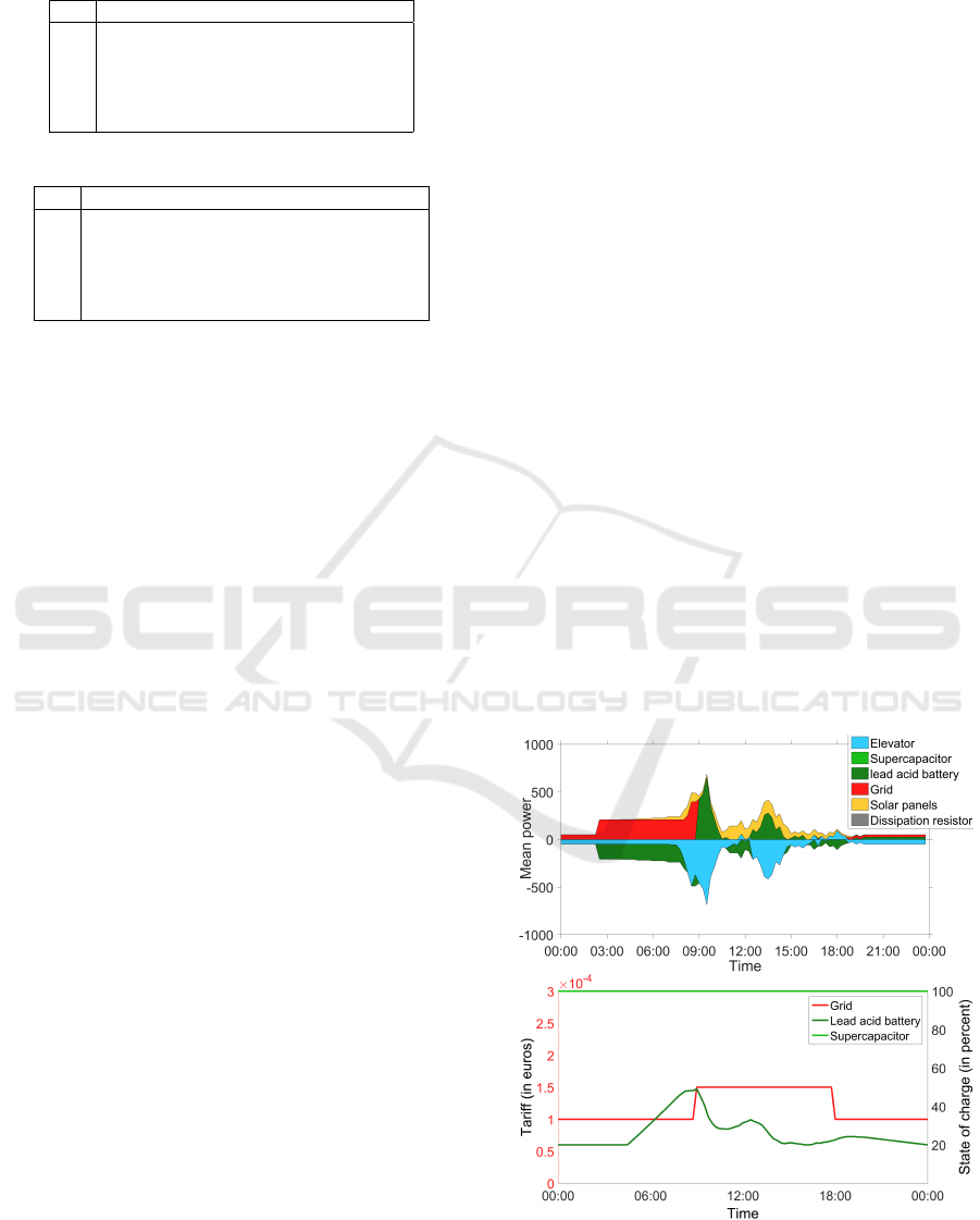
Table 2: Three LCs and their parameters.
(a) Priority orders.
MinPeaks Opportunistic Secure
P 3 3 1
S
1
4 4 3
S
2
2 2 4
S
3
1 1 2
E 5 5 5
(b) Default instructions.
MinPeaks Opportunistic Secure
P standby cons 0 W 0 W
S
1
c
minSOC
i
c
minSOC
i
c
minSOC
i
S
2
100% x
i
100%
S
3
100% x
i
x
i
E
reached, the algorithm checks if the sum of the chosen
power values is equal to zero. If not, the difference
is compensated, as much as possible, by each node
through backtracking in the tree. When the tree root is
reached, if the sum of the control vector is null, the so-
lution is kept. If not, the depth first search continues.
That way, the first found solution is the best one re-
garding the prosumers priority order, the preferences
of each prosumer and the strategic instruction.
4.3.2 Parameters Values and Objectives
This rule-based algorithm can be tuned depending
on the objective, through parameters value described
above. We cannot influence prosumers flexibilities
but we can choose priority order and default instruc-
tion. There are three versions of LC:
MinPeaks. The first controller considered seeks to
minimize power peaks purchased from control-
lable producers.
Opportunistic. The second controller considered
seeks to minimize dissipated energy and thus the
energy bill.
Secure. The third controller considered seeks to min-
imize storage units usage while guaranteeing that
storage units will be ready in case of grid failure.
Note that the Opportunistic LC’s behavior is com-
parable to a classical rule-based controller.
Priority order and default instruction associated
with each of these three controllers are shown in Ta-
ble 2. For that purpose, storage units are classified in
three categories:
• those under their minimum state of charge S
1
=
{π
i
∈ S|x
i
< c
minSOC
i
},
• those usable to absorb power peaks S
2
= {π
i
∈
S \ S
1
|p
max
i
≥ max
π
j
∈E
(−p
min
j
),
• the others S
3
= S \ (S
1
∪ S
2
).
5 RESULTS
In order to evaluate the proposed solution, we need
to compare SO plans with the results obtained by LC
following the instructions. Then, we have to compare
the different tactics between them, without strategic
instructions.
For the simulation purpose, we developed in Mat-
lab (The MathWorks Inc., 2015) a simulation engine
with dynamic time steps depending on events occur-
ring.
5.1 A Typical Strategy
Results obtained by SO, during a typical day, are il-
lustrated on Figure 3. The first sub-figure is an energy
layers plot where positive power represents power
that is injected in the energy hub (produced by pro-
sumers) and negative power represents power that is
taken from the energy hub (consumed by prosumers).
The second sub-figure presents the storage units state
of charge and the grid tariff. We can see that, when the
electricity is cheap (before 09:00), the energy is pur-
chased from the grid (in red), and stored in the battery
(in green). After 09:00, no more energy is purchased
and the energy needed is discharged from the battery.
In this situation, SO tries to take advantage of
the off-peak tariff to charge the battery and avoid to
purchase energy from the grid during the peak tariff.
We can see that the battery is charged just enough to
achieve this goal (about 40% at 09:00).
Figure 3: A typical strategic plan.
ICINCO 2016 - 13th International Conference on Informatics in Control, Automation and Robotics
26
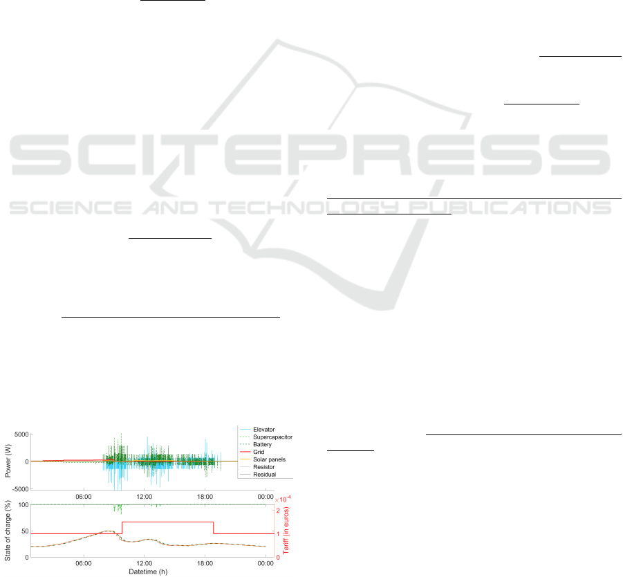
5.2 Strategic Controller Error Induced
by Aggregating Periods
In this sub-section, the point is to characterize the er-
ror made by SO when computing the objective value
(i.e. energy bill and aging costs). This error is eval-
uated (on a typical day) by comparing results of the
MinPeak LC following the strategy with results com-
puted by SO before the beginning of the day.
The plan computed before the day by SO is the
same as on Figure 3 and the corresponding MinPeaks
tactic is illustrated on Figure 4. The first sub-figure
represents the power consumption and production of
the different prosumers. We can see that the consump-
tion peaks of the elevator (in blue; that reaches 8 kW)
are absorbed by storage units (in green). While in ev-
ery cases, the maximum power peak purchased from
the grid is under 400 W, that is far less than 8 kW. The
second sub-figure shows the evolution of the storage
units state of charge and the grid tariff. In brown, we
can see the strategic instructions that are quite well
followed by the battery.
Now, let us compare numeric results of LC and
SO. As the accuracy of SO depends on 1) charging
and discharging yields of storage units, and 2) fore-
casts accuracy. We decided to consider ideal yields
(100 % and realistic yields (90 %). On the other hand,
forecasts are exact as described in sub-section 4.1.2.
Table 3 summarizes the results obtained by SO and by
the MinPeaks LC following the instructions, in three
cases.
When storage units yields are ideal, the energy bill
and the amount of energy purchased obtained by the
strategy are very close to ones obtained by the tac-
tic. Both values are less than 3 % higher with tactic
than with strategy. Though all parameters are ideal,
this small error is due to the energy aggregation in
15 mn periods into forecasts. Indeed, when sum-
ming positive and negative energy values over a pe-
riod, only the difference is kept. Then, SO take into
account only this small amount of energy to purchase
(or discharge). In reality, if production occurs be-
fore consumption, produced energy is stored and dis-
Figure 4: MinPeaks LC following strategy.
charged later to supply consumption. But, if con-
sumption occurs before production, the energy has to
be found elsewhere before the production could be
stored. When yields are ideal and storage units not
empty, that has no impact on the energy bill. But
when storage units are empty the energy has to be
purchased and that explains the small differences ob-
served above. On the other hand, the aging cost com-
puted by LC is far bigger than those estimated by the
SO because the latter did not take into account power
peaks. Indeed, to achieve instructions at the end of
a strategic period, LC cannot always charge storage
units with average power computed from the instruc-
tion. It has to absorb consumption and production
peaks, and thus to charge and discharge storage units
many times within the period. The amount of energy
charged into and discharged from storage units is thus
far bigger (about 14 times in this case) than computed
by SO.
Now let us look at the impact of realistic yields
on these results. We can see that, in the three met-
rics, results are worse than before. The reason is that
non ideal yields drive non null energy losses. Thus,
the above mentioned discrepancy due to aggregation
is emphasized in presence of non ideal yield.
In order to make SO take into account almost
all energy has to transit through storage units, we
integrate the impact of storage units yield into
consumption forecasts of prosumers in E. The strat-
egy becomes pessimistic because not all energy goes
through storage units. But the yield taken into account
in forecasts becomes a tunable parameter for the pes-
simistic prediction. Moreover, re-computing a strat-
egy every hour prevents LC to deviate too far away
from the target, even if the strategy is not perfectly
accurate. In this experiment, we choose a yield value
of 0.9, that is the real storage units yield. We can see
that the error of SO is really reduced compared to the
previous experiment. That also improves LC results,
especially on aging costs.
The last thing that has to be explained in the table
is: why do tactic aging costs are higher when yields
are ideal than when yields are realistic and when fore-
casts take yields into account? Aging costs are higher
in the former because, the battery is emptied at the be-
ginning of some periods and the supercapacitor has to
supply the elevator before being refilled by produced
energy. On the other hand, when the strategy is pes-
simistic, this situation occurs less frequently. Since
supercapacitors are much more expensive than regu-
lar batteries, aging costs in the first experiment are
higher than in the third one.
The Sourcing Problem - Energy Optimization of a Multisource Elevator
27
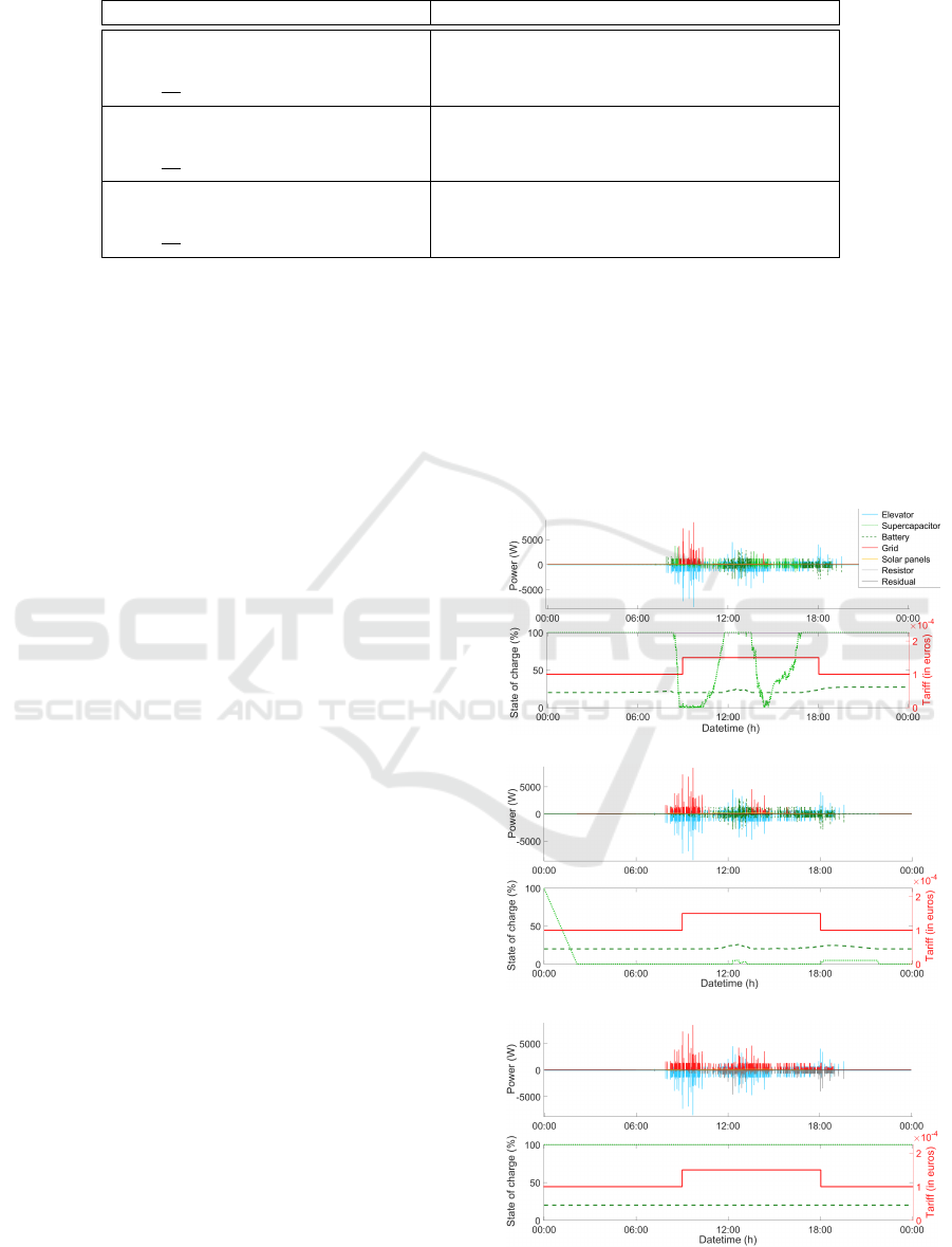
Table 3: Strategical and tactical results with different yields.
view point yield forecast energy bill aging costs energy purchased
SO 100 % exact 0.1164 e 0.0097 e 1164.3 Wh
LC 100 % exact 0.1198 e 0.1318 e 1187.8 Wh
ratio
LC
SO
100 % exact 1.03 13.59 1.02
SO 90 % exact 0.1382 e 0.0104 e 1382.2 Wh
LC 90 % exact 0.1745 e 0.3285 e 1640.5 Wh
ratio
LC
SO
90 % exact 1.26 31.59 1.19
SO 90 % exact + yield 0.1706 e 0.0117 e 1705.7 Wh
LC 90 % exact + yield 0.1655 e 0.1015 e 1654.5 Wh
ratio
LC
SO
90 % exact + yield 0.97 8.67 0.97
5.3 Three Tactics, One Strategy
Let us compare results of the different LCs, averaged
over fifty elevator usage samples drawn. For this pur-
pose, we use an additional Key Performance Indica-
tor (KPI) that is the net daily gain g
net
. Let: c
ebill
be
the energy bill of the whole day, c
0
be the energy bill
that would have been obtained without storage units,
c
aging
be the aging cost associated to the storage units
usage that have been done during the day. Moreover,
the initial state of charge of storage units are: 20%
for the battery and 100% for the supercapacitor. But
depending on the controller, final states of charge can
be different. Then we note c
soc
the cost associated
to refill (or empty) storage units to match their ini-
tial state of charge. We consider that corresponding
energy is purchased (or sold) during off-peak hours.
Then, g
net
= −(c
ebill
− c
0
+ c
aging
+ c
soc
) is an addi-
tional KPI for the following experiments.
First of all, let us look at Figures 5(a), 5(b) and
5(c) that allow us to compare the three different tac-
tics, without any strategy.
Figure 5(a) corresponds to the MinPeaks LC and
we can see that there are a few power peaks from the
grid at the beginning of the day. This is because not
enough energy was produced before consumption, so
energy had to be purchased to supply the elevator.
Moreover at the end of the day, the battery is not at
its minimum state of charge and the supercapacitor is
full.
Figure 5(b) corresponds to the Opportunistic LC.
With this tactic, all available energy is used as soon as
possible, thus the supercapacitor supplies the elevator
at the beginning of the day and is emptied. Then, there
are many power peaks purchased from the grid in the
morning and in the middle of the afternoon.
Figure 5(c) corresponds to the Secure LC. This
tactic purchases from the grid all energy needed to
preserve storage units from aging. The supercapaci-
tor, that allows the elevator to travel during grid fail-
ures, is maintained full. The battery, that has to sup-
ply supercapacitor during grid failures, is maintained
at its minimum state of charge.
Now, let us look at numerical results of these
three tactics and of the MinPeaks Controller follow-
ing strategy. The latter is illustrated on Figure 4.
Please note that a LC on its own does not take into
account electricity tariff at all. The c
0
value, in this
example, corresponds to the c
bill
value of the Secure
(a) MinPeaks LC.
(b) Opportunistic LC.
(c) Secure LC.
Figure 5: LC on their owns.
ICINCO 2016 - 13th International Conference on Informatics in Control, Automation and Robotics
28

Table 4: Net daily gain of different tactics.
SO LC p
max
c
ebill
c
aging
c
soc
g
net
X MinPeaks 317.7 0.13 0.12 0.00 0.00
7 MinPeaks 7839 0.19 0.51 -0.03 -0.42
7 Opport. 8627 0.12 0.07 0.01 0.04
7 Secure 8775 0.24 0.00 0.00 0.00
LC: c
0
= 0.24 e.
On simulated days, we can see that the only ef-
ficient way to reduce the maximum power peak pur-
chased from the grid is the MinPeaks Controller fol-
lowing the strategy. That way, the purchasing peak is
less than 5% of the maximum possible power peak.
The tactics on their own do not absorb power peaks,
because a predictive strategy is necessary to achieve
such a goal. On the other hand, the MinPeaks Con-
troller following the strategy only succeeds to com-
pensate aging costs by a gain on the energy bill. Thus,
its net daily gain is null in this context. Please note
that, if the gap between on- and off-peak hourly cost
grows, the net daily gain of this tactic following the
strategy also increases.
If the MinPeaks LC is on its own (for example
during a long network failure), the net daily gain be-
comes negative but the number of (and the maximum)
power peaks stays below the other controllers alone.
However, if the goal is only to minimize the net
daily gain, without taking into account power peaks,
the Opportunistic LC alone is the best (as far as the
ratio between the high/low prices is moderate).
Finally, the Secure tactic does not use storage
units at all and thus, has a higher energy bill, but a
null aging cost.
6 CONCLUSIONS
In this paper we formalize what we call the sourc-
ing problem and its application to a multisource ele-
vator. We give a method to solve it, composed of a
Local Controller coupled with a Strategic Optimizer.
That allows us to tackle real-time issues while taking
into account long-term objectives based on forecasts.
A linear formulation allows us to compute a strategy
and a centralized rule-based algorithm gives us a tac-
tic. Three Local Controller parametrizations are il-
lustrated, and one will choose the most adapted to its
studied energy hub.
A legitimate criticism of this work could be that
gains in euros are very low. First, let us recall that
these results are for a unique elevator, while in prac-
tice several elevators could share the same battery.
Second, reducing power consumption peaks could be
very useful to be demand-response aware and to re-
spect future energy limitation laws. In those cases,
minimizing the energy bill is only an appreciable ad-
dition to the consumption peaks minimization. For
the multisource elevator use case, having storage units
allows the elevator to evacuate disabled people in case
of fire. Using these storage units to minimize the en-
ergy bill could amortize the investment. Third, en-
ergy prices are going to increase in future years, as
will storage units performances. That will also in-
crease the benefit of this solution. Finally, the pro-
posed solution can be applied to other multisource
systems where it can be much more profitable. In fact,
as the consumption increases, the profitability also in-
creases, especially if reselling energy is possible.
On the other hand, we will have to compare the
cost of maintaining our rather complex solution, re-
garding the customer value in each use case. If the
maximum power peak purchased from the grid is not
an issue and the energy tariff considered is a typi-
cal French peak/off-peak tariff, the Opportunistic LC
(or a similar classical rule-based controller) should be
used.
As future work, we will study our method robust-
ness to forecast uncertainties. This is a critical issue
and studying it could allow us to give performance
guarantees to potential customers. A sensibility study
of controller parameters will also be conducted. Fi-
nally, a real-life experiment, in a building equipped
with a BMS, would worth being conducted.
ACKNOWLEDGEMENTS
This work has been conducted as part of the Arrow-
head European project and has been partially funded
by the Artemis/Ecsel Joint Undertaking, supported by
the European Commission and French Public Author-
ities, under grant agreement number 332987.
REFERENCES
Bilbao, E. and Barrade, P. (2012). Optimal energy man-
agement of an improved elevator with energy storage
capacity based on dynamic programming. In Energy
Conversion Congress and Exposition (ECCE), 2012
IEEE, page 3479–3484.
Boutin, V., Desdouits, C., Louvel, M., Pacull, F., Vergara-
Gallego, M. I., Yaakoubi, O., Chomel, C., Crignon,
Q., Duhoux, C., Genon-Catalot, D., Lefevre, L.,
Pham, T. H., and Pham, V. T. (2014). Energy optimi-
sation using analytics and coordination, the example
of lifts. In Emerging Technology and Factory Automa-
tion (ETFA), 2014 IEEE, pages 1–8. IEEE.
Desdouits, C., Alamir, M., Boutin, V., and Pape, C. L.
(2015). Multi-source elevator energy optimization
The Sourcing Problem - Energy Optimization of a Multisource Elevator
29

and control. In European Control Conference (ECC),
EUCA 2015. EUCA.
GNU (2014). GNU Linear Programming Kit, version 4.54.
http://www.gnu.org/software/glpk/glpk.html.
Paire, D., Simoes, M. G., Lagorse, J., and Miraoui, A.
(2010). A real-time sharing reference voltage for hy-
brid generation power system. In Industry Applica-
tions Society Annual Meeting (IAS), 2010 IEEE, pages
1–8. IEEE.
Sachs, H. M. (2005). Opportunities for elevator energy ef-
ficiency improvements. Technical report, American
Council for an Energy-Efficient Economy Washing-
ton, DC.
The MathWorks Inc. (2015). Matlab 2015b. The Math-
Works Inc., Natick, Massachusetts, United States.
Tominaga, S., Suga, I., Araki, H., Ikejima, H., Kusuma, M.,
and Kobayashi, K. (2002). Development of energy-
saving elevator using regenerated power storage sys-
tem. In Power Conversion Conference, 2002. PCC-
Osaka 2002. Proceedings of the, volume 2, pages
890–895. IEEE.
ICINCO 2016 - 13th International Conference on Informatics in Control, Automation and Robotics
30
