
Mode Combining and -Splitting in Optical MIMO Transmission using
Photonic Lanterns
Andreas Ahrens and Steffen Lochmann
Hochschule Wismar, University of Technology, Business and Design,
Philipp-Müller-Straße 14, 23966 Wismar, Germany
Keywords:
Multiple-Input Multiple-Output System, Singular-Value Decomposition, Photonic Lantern, Optical MIMO
Transmission.
Abstract:
Within the last years the multiple-input multiple-output (MIMO) technology has revolutionized the optical
fibre community. Theoretically, the concept of MIMO is well understood and shows some similarities to wire-
less MIMO systems. However, practical implementations of optical components are in the focus of interest
of substantial research. Optical couplers have long been used as passive optical components also being able
to combine or split SISO (single-input single-output) data transmission. They have been proven to be well
suited for the optical MIMO (multiple-input multiple-output) transmission despite their insertion losses and
asymmetries. Nowadays, next to optical couplers, Photonic Lanterns (PLs) have attracted a lot of attention in
the research community as they offer the benefit of a low loss transition from the input fibers to the modes
supported by the waveguide at its output. Therefore they seem to be highly beneficial for optical MIMO com-
munication. In this contribution mode coupling and splitting devices such as PLs and fusion couplers have
been analysed in a testbed with regard to their respective MIMO suitability. Based on the obtained results, a
simplified time-domain MIMO simulation model including PLs for mode-combining at the transmitter side as
well as mode-splitting at the receiver side is elaborated. Our results obtained by the simulated bit-error rate
(BER) performance show that PLs are well suited for the optical MIMO transmission.
1 INTRODUCTION
The growing demand of bandwidth particularly
driven by the developing Internet has been satisfied
so far by optical fibre technologies such as Dense
Wavelength Division Multiplexing (DWDM), Polar-
ization Multiplexing (PM) and multi-level modula-
tion. These technologies have now reached a state
of maturity (Winzer, 2012). The only way to fur-
ther increase the available data rate is now seen in the
area of spatial multiplexing (Richardson et al., 2013),
which is well-established in wireless communications
(Tse and Viswanath, 2005; Kühn, 2006). Nowa-
days several novel techniques such as Mode Group
Diversity Multiplexing (MGDM) (Franz and Bülow,
2012) or Multiple-InputMultiple-Output (MIMO) are
in the focus of interest (Singer et al., 2008). Among
these techniques, the concept of MIMO transmission
(Kühn, 2006; Foschini, 1996) over multi-mode fibers
has attracted increasing interest in the optical fiber
transmission community, targeting at increased fiber
capacity (Singer et al., 2008; Aust et al., 2012). The
fiber capacity of a multi-mode fiber is limited by the
modal dispersion compared to single-mode transmis-
sion where no modal dispersion except for polariza-
tion exists. The description of the optical MIMO
channel has attracted attention and reached a state of
maturity (Singer et al., 2008; Hsu et al., 2006; Bülow
et al., 2011).
However, the realization of the optical MIMO
channel requires substantial further research regard-
ing mode combining, mode maintenance and mode
splitting (Schöllmann and Rosenkranz, 2007; Schöll-
mann et al., 2008). Hence, Photonic Lanterns (PLs)
have attracted a lot of attention in the research com-
munity (Leon-Saval et al., 2014; Huang et al., 2015;
Fontaine et al., 2013). Compared to other passive de-
vices used for mode combining and mode splitting
such as optical couplers, PLs offer the benefit of a low
loss transition from the input fibers to the modes sup-
ported by the waveguide at its output which makes
such devices very attractive for optical MIMO com-
munication.
In this contribution mode coupling and splitting
devices such as PLs and fusion couplers have been
analysed in a testbed with regard to their respective
Ahrens, A. and Lochmann, S.
Mode Combining and -Splitting in Optical MIMO Transmission using Photonic Lanterns.
DOI: 10.5220/0005944600890096
In Proceedings of the 6th International Joint Conference on Pervasive and Embedded Computing and Communication Systems (PECCS 2016), pages 89-96
ISBN: 978-989-758-195-3
Copyright
c
2016 by SCITEPRESS – Science and Technology Publications, Lda. All rights reserved
89
MIMO suitability. Based on the obtained results, a
simplified time-domain MIMO simulation model in-
cluding PLs for mode-combining at the transmitter
side as well as mode-splitting at the receiver side is
elaborated. Our results obtained by the simulated
BER performance show that PLs are well suited for
the optical MIMO transmission.
The remaining part of this paper is structured as
follows: Section 2 introduces the practical issues of
optical MIMO. The newly developed concept of the
PL and the resulting system model are analyzed in
section 3. The associated performance results are pre-
sented and interpreted in section 4. Finally, section 5
provides some concluding remarks.
2 PRACTICAL ISSUES OF
OPTICAL MIMO
An optical MIMO system can be formed by feeding
different sources of light into the fiber. These sources
of light activate different optical modes. Theoreti-
cally, it can be done by using two single-mode fibers
(Ahrens and Lochmann, 2013) as shown in Fig. 1.
Practically, a possible solution for feeding different
sources of light into the fibre can be provided by op-
tical couplers (see Fig. 2). It is well known that op-
tical couplers may show a strong mode selective be-
havior. In general this behavior depends on the fab-
rication technique. Although the term ’mode selec-
tivity’ is usually referred to the unwanted coupling
ratio’s dependency on the launching conditions, we
can make use of this parameter to control or better to
maintain the mode groups within such a device. Dif-
ferent kinds of couplers have been studied in (Ahrens
Figure 1: Transmitter side configuration with center and
offset light launch condition.
(low order mode path)
(high order mode path)
1
2
3
Figure 2: Transmitter-side coupler for launching different
sources of light into the multi-mode fibre (MMF).
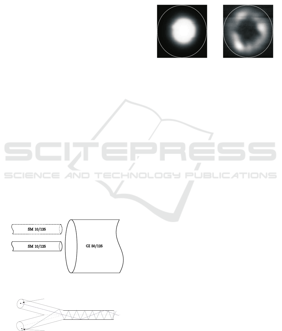
and Lochmann, 2013). A measured mean power dis-
tribution pattern of an asymmetric fusion coupler at
the coupler output is depicted in Fig. 3. Here, dif-
ferent launching conditions were used for creating in-
dividual modes, which are subsequently combined by
the coupler. As shown in Fig. 3 the fundamental mode
Figure 3: Measured mean power distribution pattern as a
function of the light launch position at an operating wave-
length of λ = 1550nm (left: eccentricity δ = 0µm, right: ec-
centricity δ = 15µm); the dotted line represents the 50µm
core size.
as well as the higher-order mode groups are spatially
well separated. Using these couplers for mode com-
bining at the transmitter side and mode splitting at the
receiverside, a simple MIMO direct detection scheme
can be formed. However, the demand for higher data
rates requires high-level modulation formats, which
are not feasible by direct detection receivers.
Photonic Lanterns, which have attracted a lot of
attention in the research community, may overcome
this disadvantage. Besides using integrated optical
chips they are mostly produced by fusing and tapering
single-mode fibres (Leon-Saval et al., 2014; Huang
et al., 2015; Fontaine et al., 2013), which are placed
in a low refractive index capillary. The process is
controlled in such a way that the taper matches the
dimensions of the following few-mode fibre (FMF).
Now, the input single-mode fibre channels create indi-
vidual mode-patterns at the output of the PL. Having
an ideal FMF channel, these individual mode-patterns
are re-transformed into the independent single-mode
fibre (SMF) channels.
Fig. 4 shows exemplarily three measured mean
power distribution patterns at the output of the PL as
an example of the investigated 6-port PL. Thereby,
the creation of the different mode patterns capable
of carrying individual data channels has been veri-
fied. Since the FMF dimension supports only four
modes, the obtained patterns must consist of super
positioned modes as demonstrated in (Huang et al.,
2015) or (Fontaine et al., 2013), too.
In comparison to the fusion coupler shown in
Fig. 3 the PL does not show well separated mode
patterns. However, the concept of activating individ-
ual modes offers the possibility of coherent transmis-
sion combined with high-level modulation schemes
SPCS 2016 - International Conference on Signal Processing and Communication Systems
90
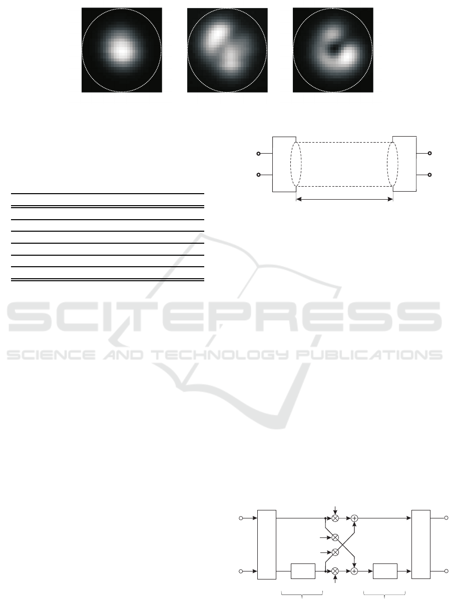
Figure 4: Measured mean power distribution patterns at the output of the PL using different input SMFs at an operating
wavelength of λ = 1550nm; the dotted line represents the 30µm core size.
such as 16-QAM (quadrature amplitude modulation)
or 256-QAM.
Table 1: Comparison of the investigated asymmetric fusion
coupler and the PL with respect to insertion losses (in dB).
Insertion Loss Fusion Coupler Photonic Lantern
a
12
0,1 6,7
a
13
8,1 6,7
a
14
−− 4,2
a
15
−− 4,1
a
16
−− 7,0
a
17
−− 4,1
For the evaluation of the whole MIMO concept,
the component dependent losses play an important
role and must be characterized. Tab. 1 compares the
investigated asymmetric fusion coupler and the PL
with respect to their insertion losses.
Although the fusion coupler may form well sepa-
rated mode patterns, its insertion losses exhibit a high
asymmetry. However, the PL which may theoretically
achieve a 0 dB insertion loss, shows notable vari-
ations, too. Further technology improvements may
overcome these variations.
Now, the carried out measurements form the basis
for the development of a time domain MIMO simu-
lation model, which takes the mode combining and
mode splitting components into account.
3 TIME-DOMAIN SIMULATION
MODEL
In this section the MIMO transmission scheme is in-
troduced. For simplification a (2×2) MIMO scheme
is analyzed. Here, an ideal (2×2) PL is considered,
where SMFs are connected with the respective inputs
Tx−1 as well as Tx−2 as shown in Fig. 5. The map-
ping of the incoming LP
01
modes by the PL can be
described by the corresponding coupling matrix
K
TX
=
1 0
0 1
(1)
Photonic Lantern
Photonic Lantern
LP
01
LP
01
LP
01
LP
01
Tx-1
Tx-2
Rx-1
Rx-2
ℓ
Figure 5: Multi-mode MIMO transmission using Photonic
Lantern for mode combining and splitting.
resulting in the mode LP
01
at the output 1 as well as
in the mode LP
11
at the output 2 (see Fig. 6). Further-
more, in this work it is assumed that the coupling ma-
trix of the receiver side PL equals the coupling matrix
of the transmitter side, i. e., K
RX
= K
TX
. The corre-
sponding system model is depicted in Fig. 6.
Here, it is worth noting that under practical as-
sumptions the output of the PL in Fig. 6, the LP
01
-
and LP
11
mode may appear as superposition modes
as highlighted in section 2.
In the time-domain, the impulse responses of the
FMF channel are given as follows
g
11
(t) = k
11
δ(t) g
12
(t) = k
12
δ(t −∆τ/2)
g
21
(t) = k
21
δ(t −∆τ/2) g
22
(t) = k
12
δ(t −∆τ)
describing the mode-coupling of the underlying chan-
nel. Herein, the parameter ∆τ describes the differen-
tial mode delay between the fundamental mode LP
01
and the mode LP
11
, which is identified to be ∆τ = 200
ps for the considered fibre length of 2 km. The opti-
cal field coupling coefficients of the underlying FMF
Photonic Lantern
Photonic Lantern
LP
01
LP
01
LP
01
LP
01
LP
01
LP
01
LP
11
LP
11
Tx-1
Rx-1
Tx-2
Rx-2
ℓ/2
ℓ/2
∆τ/2
∆τ/2
k
1 1
k
2 2
k
2 1
k
1 2
Figure 6: Underlying MIMO-based System Model of the
fibre length ℓ.
Mode Combining and -Splitting in Optical MIMO Transmission using Photonic Lanterns
91

channel, describing the coupling from the mode LP
01
to the mode LP
11
and from the mode LP
11
to the
mode LP
01
, are given by the coupling matrix K
C
K
C
=
k
11
k
12
k
21
k
22
, (2)
with the parameter k
νµ
to be determined. Since no
power-loss is assumed, the coupling coefficients have
to fulfill the following condition for the considered
(2×2) MIMO system
L
∑
ν=1
k
2
νµ
= 1 for µ = 1,2,... , L and L = 2 .
(3)
Finally, the effect of the chromatic dispersion is not
analyzed in this contribution since the focus of this
simulation is on the MIMO characteristic. However,
it can be taken into account by a simple convolution
of the impulse responses g
νµ
(t) with a Gaussian dis-
tribution modelling the chromatic dispersion.
The mode-coupling along the optical channel to-
gether with the PL at the transmitter as well as the
receiver side is forming a MIMO system, as given in
Fig. 7. Here, each optical input within the multi-mode
fiber is fed by a system with identical mean proper-
ties with respect to transmit filter and pulse frequency
f
T
= 1/T
s
. Rectangular pulses are used for transmit
and receive filtering, i. e. g
s
(t) and g
ef
(t) in order to
form the overall impulse response g
(νµ)
(t) as follow
g
(νµ)
(t) = g
s
(t) ∗g
νµ
(t) ∗g
ef
(t) . (4)
The MIMO block diagram of the transmission model
is shown in Fig. 8. When considering a frequency-
selective MIMO link, composed of n
T
optical in-
puts and n
R
optical outputs, the resulting electrical
discrete-time block-oriented system can be modelled
by
u = H·c+ w . (5)
In (5), c is the (N
T
×1) transmitted signal vector con-
taining the input symbols transmitted over n
T
optical
inputs in K consecutive time slots, i. e., N
T
= Kn
T
.
u
TX 1
(t)
u
TX 2
(t)
u
RX 1
(t)
u
RX 2
(t)
g
11
(t)
g
21
(t)
g
12
(t)
g
22
(t)
Figure 7: Electrical (2×2) MIMO system model.
transmit vector
receive vector
noise vector
c
u
H
w
Figure 8: Transmission system model.
This vector can be decomposed into n
T
transmitter-
specific signal vectors c
µ
according to
c =
c
T
1
,... ,c
T
µ
,... ,c
T
n
T
T
. (6)
In (6), the (K × 1) input-specific signal vector c
µ
transmitted by the optical input µ (with µ = 1,.. ., n
T
)
is modelled by
c
µ
=
c
1µ
,... ,c
kµ
,... ,c
Kµ
T
. (7)
The (N
R
× 1) received signal vector u, defined in
(5), can again be decomposed into n
R
output-specific
signal vectors u
ν
(with ν = 1,.. ., n
R
) of the length
K + L
c
, i.e., N
R
= (K + L
c
)n
R
, and results in
u =
u
T
1
,... ,u
T
ν
,... ,u
T
n
R
T
. (8)
By taking the (L
c
+ 1) non-zero elements of the re-
sulting symbol rate sampled overall channel impulse
response g
(νµ)
(t) between the µth input and νth out-
put into account, the output-specific received vector
u
ν
has to be extended by L
c
elements, compared to
the transmitted input-specific signal vector c
µ
defined
in (7). The ((K + L
c
) × 1) signal vector u
ν
received
by the optical output ν (with ν = 1,... ,n
R
) can be
constructed, including the extension through the mul-
tipath propagation, as follows
u
ν
=
u
1ν
,u
2ν
,... ,u
(K+L
c
)ν
T
. (9)
Similarly, in (5) the (N
R
×1) noise vector w results in
w =
w
T
1
,... ,w
T
ν
,... ,w
T
n
R
T
. (10)
The vector w of the additive, white Gaussian noise
(AWGN) can still be decomposed into n
R
transmitter-
specific signal vectors w
ν
(with ν = 1,... ,n
R
) accord-
ing to
w
ν
=
w
1ν
,w
2ν
,... ,w
(K+L
c
)ν
T
. (11)
Finally, the (N
R
×N
T
) system matrix H of the block-
oriented system model, introduced in (5), results in
H =
H
11
... H
1n
T
.
.
.
.
.
.
.
.
.
H
n
R
1
··· H
n
R
n
T
, (12)
and consists of n
R
n
T
single-input single-output
(SISO) channel matrices H
νµ
(with ν = 1, ... ,n
R
and
SPCS 2016 - International Conference on Signal Processing and Communication Systems
92

replacements
p
ξ
1 k
p
ξ
2 k
w
1 k
w
2 k
c
1 k
c
2 k
y
1 k
y
2 k
Figure 9: SVD-based layer-specific transmission model.
µ = 1,... ,n
T
). Every of these matrices H
νµ
with the
dimension ((K + L
c
) × K) describes the influence of
the channel from transmitter µ to receiver ν including
transmit and receive filtering, i.e. g
(νµ)
(t). The chan-
nel convolution matrix H
νµ
between the µth input and
νth output is obtained by taking the (L
c
+ 1) non-zero
elements of resulting symbol rate sampled overall im-
pulse response g
(νµ)
(t) into account and results in:
H
νµ
=
h
0
0 0 ··· 0
h
1
h
0
0 ···
.
.
.
h
2
h
1
h
0
··· 0
.
.
. h
2
h
1
··· h
0
h
L
c
.
.
. h
2
··· h
1
0 h
L
c
.
.
. ··· h
2
0 0 h
L
c
···
.
.
.
0 0 0 ··· h
L
c
. (13)
The interference, which is introduced by the off-
diagonal elements of the channel matrix H, requires
appropriate signal processing strategies. A popular
technique is based on the singular-value decomposi-
tion (SVD) of the system matrix H, which can be
written as H = S · V· D
H
, where S and D
H
are uni-
tary matrices and V is a real-valued diagonal matrix
of the positive square roots of the eigenvalues of the
matrix H
H
H sorted in descending order
1
. The SDM
(spatial division multiplexing) MIMO data vector c is
now multiplied by the matrix D before transmission.
In turn, the receiver multiplies the received vector u
by the matrix S
H
. Thereby neither the transmit power
nor the noise power is enhanced. The overall trans-
mission relationship is defined as
y = S
H
(H·D·c+ w) = V·c+ ˜w. (14)
As a consequence of the processing in (14), the
channel matrix H is transformed into independent,
non-interfering layers having unequal gains (Pankow
et al., 2011; Raleigh and Cioffi, 1998).
In MIMO communication, singular-value decom-
position (SVD) has been established as an efficient
1
The transpose and conjugate transpose (Hermitian) of
D are denoted by D
T
and D
H
, respectively.
concept to compensate the interferences between the
different data streams transmitted over a dispersive
channel: SVD is able to transfer the whole sys-
tem into independent, non-interfering layers exhibit-
ing unequal gains per layer as highlighted in Fig. 9,
where as a result weighted additive, white Gaussian
noise (AWGN) channels appear.
Analyzing the considered (2×2) MIMO system,
the data symbols at the time k (with k = 1,2,. . .,K),
i. e. c
1k
and c
2k
are weighted by the positive square
roots of the eigenvalues of the matrix H
H
H, i. e.
p
ξ
1k
and
p
ξ
2k
. Finally, some noise is added,
i. e. w
1k
and w
2k
. Here it is worth noting that the
the number of readily separable layers is limited by
min(n
T
,n
R
). Therefore in this work the maximum
number of layers is given by L = 2.
In general the quality criterion for transmission
systems can be expressed by using the signal to noise
ratio (SNR) at the detector input as follows
ρ =
(half vertical eye opening)
2
noise power
=
(U
A
)
2
P
R
, (15)
where U
A
and P
R
correspond to one quadrature com-
ponent. Considering a layer-based MIMO system
with a given SNR ρ
(ℓ,k)
for each layer ℓ (with ℓ =
1,2, . ..,L) and time k (with k = 1,2,. ..,K) and a M-
ary quadrature amplitude modulation (QAM), the bit-
error rate (BER) probability is given by
P
(ℓ,k)
BER
=
2
log
2
M
ℓ
1−
1
√
M
ℓ
er fc
s
ρ
(ℓ,k)
2
.
(16)
This BER is averaged over all time slots and activated
layers taking different modulation sizes at each layer
into account. For QAM modulated signals the aver-
age transmit power per layer can be expressed as
P
s,ℓ
=
2
3
U
2
s,ℓ
(M
ℓ
−1) . (17)
Intuitively the total available transmit power P
s
is
equally split between the L activated layers, and hence
the layer-specific transmit power is given by P
s,ℓ
=
P
s
/L, influencing the half-level transmit amplitude
U
s,ℓ
for each MIMO layer.
Considering the SVD layer model, the noise
power is unchanged at the receiver. However, the
half vertical eye openings U
A
at each time slot k
(with k = 1,2,.. . ,K) and layer ℓ (with ℓ = 1,2, . .., L)
are influenced by the singular values so that U
(ℓ,k)
A
=
p
ξ
ℓ,k
U
s,ℓ
holds and the corresponding SNR values
are given by
ρ
(ℓ,k)
SVD
=
ξ
ℓ,k
U
2
s,ℓ
P
R
=
3ξ
ℓ,k
L(M
ℓ
−1)
E
s
N
0
, (18)
Mode Combining and -Splitting in Optical MIMO Transmission using Photonic Lanterns
93

with E
s
being the transmit symbol energy and the pa-
rameter N
0
describing the noise power spectral den-
sity. The overall bit-error rate of the uncoded MIMO
system is largely determined by the layer with the
highest BER. In order to balance the bit-error rates,
the mean of choice is to equalize the SNR values ρ
(ℓ,k)
SVD
over all layers and time-slots. This is clearly not the
optimal solution for minimizing the overall BER but
it is easy to implement and not far away from the
optimum as shown in (Ahrens and Benavente-Peces,
2009). Therefore, the half-level transmit amplitude
U
s,ℓ
is adjusted on each layer by multiplying it with
√
p
ℓ,k
in order to apply the power allocation (PA)
scheme. Consequently, the half vertical eye opening
of the received symbols becomes
U
(ℓ,k)
A,PA
=
√
p
ℓ,k
q
ξ
ℓ,k
U
s,ℓ
. (19)
With this adjustment the SNR values are resulting in
ρ
(ℓ,k)
PA
= p
ℓ,k
ρ
(ℓ,k)
SVD
. (20)
In the SVD-based model the singular values are vary-
ing for each time slot. Consequently, power alloca-
tion should be able to balance the BER’s on all layers
L and given time slots per block K. Therefore, the
overall transmit power after PA needs to be the same
as without PA and thus
P
s
=
1
K
K
∑
k=1
L
∑
ℓ=1
p
ℓ,k
·P
s,ℓ
=
P
s
KL
K
∑
k=1
L
∑
ℓ=1
p
ℓ,k
(21)
has to be guaranteed, resulting in the condition
K ·L =
L
∑
ℓ=1
K
∑
k=1
p
ℓ,k
(22)
for the total available transmit power. As a result, the
power allocation factors for layer and time-based PA
in SVD systems can be calculated as follows
p
(LT−SVD)
ℓ,k
=
(M
ℓ
−1)
ξ
ℓ,k
K ·L
∑
L
ν=1
∑
K
κ=1
(M
λ
−1)
ξ
ν,κ
(23)
and guarantee the above mentioned equal-SNR sce-
nario for all activated layers and time slots per trans-
mitted block (Ahrens et al., 2015). An illustration of
the resulting SNRs of the proposed PA schemes for
SVD systems is depicted in Fig. 10.
4 PERFORMANCE ANALYSIS
For comparing the different MIMO configurations, a
fixed transmission bit rate is analysed. Furthermore,
for numerical analysis it is assumed, that each optical
layer ℓ
time k
layer ℓ
time k
Figure 10: Illustration of the remaining SNRs in SVD sys-
tems without applying PA (left) and with combined layer
and time PA (right). The color black refers to high and white
to low SNR values.
input within the multi-mode fiber is fed by a system
with identical mean properties with respect to trans-
mit filtering and pulse frequency f
T
= 1/T
s
. Rectan-
gular pulses are used for transmit and receive filter-
ing. The average transmit power is supposed to be
P
s
= 1V
2
. This equals 1 W at a linear and constant
resistance of 1Ω. As an external disturbance a white
Gaussian noise with power spectral density N
0
is as-
sumed (Pankow et al., 2011). Tab. 2 highlights the
different transmission modes to be investigated when
minimizing the overall BER at a fixed data rate.
Table 2: Parameters for bitloading: Investigated QAM
transmission modes for fixed transmission bit rate.
throughput layer 1 layer 2
4 bit/s/Hz 16 0
4 bit/s/Hz 4 4
In order to transmit at a fixed data rate while main-
taining the best possible integrity, i. e. bit-error rate
(BER), an appropriate number of MIMO layers has
to be used, which depend on the specific QAM con-
stellation size as well as the layer-specific weighting
factors, i.e.
p
ξ
1k
and
p
ξ
2k
.
The optical field coupling coefficients of the un-
derlying FMF channel shall be given as follows
K
C1
=
0,83 0,54
0,54 0,83
(24)
and
K
C2
=
0,94 0,31
0,31 0,94
, (25)
with the coupling matrix K
C1
defining 30% crosstalk
and the matrix K
C2
defining 10% channel crosstalk.
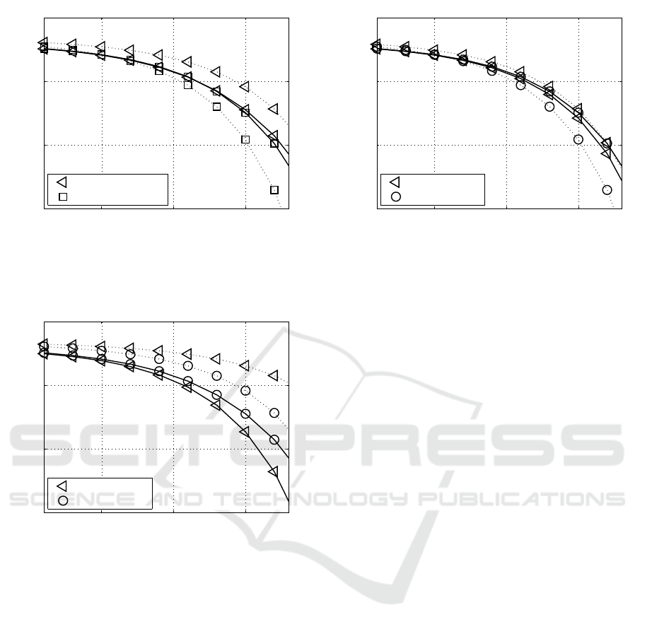
For a given MIMO configuration the correspond-
ing BER performance is depicted in Fig. 11. The pa-
rameters are chosen as follows: the pulse frequency
equals f
T
= 5.00 GHz and the differential mode de-
lay is identified to be ∆τ = 200 ps for the considered
fibre length of 2 km.
As shown by the BER results, the achievable per-
formance of the MIMO system is strongly affected by
the channel crosstalk. Using SVD, the singular val-
ues are ordered in descending order. Thereby only the
strongest layer should be used for the data transmis-
sion with appropriate QAM modulation levels in the
SPCS 2016 - International Conference on Signal Processing and Communication Systems
94
5 10 15
10
−6
10
−4
10
−2
10
0
10 ·log
10
(E
s
/N
0
) (indB) →
bit-error rate →
K
C1
, 30% crosstalk
K
C2
, 10% crosstalk
Figure 11: BER performance when activating two layers
(dotted line) as well as one layer (solid line) and using the
transmission modes introduced in Tab. 2 at different channel
couplings.
5 10 15
10
−6
10
−4
10
−2
10
0
10 ·log
10
(E
s
/N
0
) (indB) →
bit-error rate →
f
T
= 1,00 GHz
f
T
= 5,00 GHz
Figure 12: BER performance when activating two layers
(dotted line) as well as one layer (solid line) and using the
transmission modes introduced in Tab. 2 at the channel cou-
pling K
C1
.
case of high crosstalk conditions. However, in prac-
tical implementations fibres usually show only small
crosstalk values. Thus, activating two MIMO layers
becomes more and more beneficial.
Analyzing different pulse frequencies, the result-
ing BER performance is highlighted in Fig. 12 and
Fig. 13 for different parameters of the channel cou-
pling. However, considering a fixed differential mode
delay, at low pulse frequencies less intersymbol inter-
ference appears and the BER performance improves
even under high crosstalk conditions.
5 CONCLUSIONS
In this contribution mode coupling and splitting de-
5 10 15
10
−6
10
−4
10
−2
10
0
10 ·log
10
(E
s
/N
0
) (indB) →
bit-error rate →
f
T
= 1,00 GHz
f
T
= 5,00 GHz
Figure 13: BER performance when activating two layers
(dotted line) as well as one layer (solid line) and using the
transmission modes introduced in Tab. 2 at the channel cou-
pling K
C2
.
vices such as PLs and fusion couplers have been
analysed in a testbed with regard to their respec-
tive MIMO suitability. The established time-domain
MIMO simulation model proven to be a versatile tool
for the optimization of the overall MIMO transmis-
sion system shows that PLs are well suited for optical
MIMO communications.
ACKNOWLEDGEMENTS
This work has been funded by the German Ministry
of Education and Research (No. 03FH016PX3).
REFERENCES
Ahrens, A. and Benavente-Peces, C. (2009). Modulation-
Mode and Power Assignment in Broadband MIMO
Systems. Facta Universitatis (Series Electronics and
Energetics), 22(3):313–327.
Ahrens, A. and Lochmann, S. (2013). Optical Couplers in
Multimode MIMO Transmission Systems: Measure-
ment Results and Performance Analysis. In Interna-
tional Conference on Optical Communication Systems
(OPTICS), pages 398–403, Reykjavik (Iceland).
Ahrens, A., Sandmann, A., Lochmann, S., and Wang, Z.
(2015). Decomposition of Optical MIMO Systems us-
ing Polynomial Matrix Factorization. In 2nd IET In-
ternational Conference on Intelligent Signal Process-
ing, London (United Kingdom).
Aust, S., Ahrens, A., and Lochmann, S. (2012). Channel-
Encoded and SVD-assisted MIMO Multimode Trans-
mission Schemes with Iterative Detection. In Interna-
tional Conference on Optical Communication Systems
(OPTICS), pages 353–360, Rom (Italy).
Mode Combining and -Splitting in Optical MIMO Transmission using Photonic Lanterns
95

Bülow, H., Al-Hashimi, H., and Schmauss, B. (2011).
Coherent Multimode-Fiber MIMO Transmission with
Spatial Constellation Modulation. In European Con-
ference and Exhibition on Optical Communication
(ECOC), Geneva, Switzerland.
Fontaine, N. K., Leon-Saval, S. G., Ryf, R., Salazar-Gil,
J. R., Ercan, B., and Bland-Hawthorn, J. (2013).
Mode-Selective Dissimilar Fiber Photonic-Lantern
Spatial Multiplexers for Few-Mode Fiber. In 39th Eu-
ropean Conference and Exhibition on Optical Com-
munication (ECOC 2013), pages 1–3, London, United
Kingdom.
Foschini, G. J. (1996). Layered Space-Time Architecture
for Wireless Communication in a Fading Environment
when using Multiple Antennas. Bell Labs Technical
Journal, 1(2):41–59.
Franz, B. and Bülow, H. (2012). Experimental Evaluation
of Principal Mode Groups as High-Speed Transmis-
sion Channels in Spatial Multiplex Systems. IEEE
Photonics Technology Letters, 24:1363–1365.
Hsu, R. C. J., Tarighat, A., Shah, A., Sayed, A. H., and
Jalali, B. (2006). Capacity Enhancement in Coherent
Optical MIMO (COMIMO) Multimode Fiber Links.
IEEE Communications Letters, 10(3):195–197.
Huang, B., Fontaine, N. K., Ryf, R., Guan, B., Leon-Saval,
S. G., Shubochkin, R., Sun, Y., Lingle Jr, R., and Li,
G. (2015). All-Fiber Mode-Group-Selective Photonic
Lantern using Graded-Index Multimode Fibers. Op-
tics Express, 23(1):224–234.
Kühn, V. (2006). Wireless Communications over MIMO
Channels – Applications to CDMA and Multiple An-
tenna Systems. Wiley, Chichester.
Leon-Saval, S. G., Fontaine, N. K., Salazar-Gil, J. R., Er-
can, B., Ryf, R., and Bland-Hawthorn, J. (2014).
Mode-Selective Photonic Lanterns for Space-Division
Multiplexing. Optics Express, 22(1):1–9.
Pankow, J., Aust, S., Lochmann, S., and Ahrens, A. (2011).
Modulation-Mode Assignment in SVD-assisted Op-
tical MIMO Multimode Fiber Links. In 15th Inter-
national Conference on Optical Network Design and
Modeling (ONDM), Bologna (Italy).
Raleigh, G. G. and Cioffi, J. M. (1998). Spatio-Temporal
Coding for Wireless Communication. IEEE Transac-
tions on Communications, 46(3):357–366.
Richardson, D. J., Fini, J., and Nelson, L. (2013). Space
Division Multiplexing in Optical Fibres. Nature Pho-
tonics, 7:354–362.
Schöllmann, S. and Rosenkranz, W. (2007). Experimen-
tal Equalization of Crosstalk in a 2 x 2 MIMO Sys-
tem Based on Mode Group Diversity Multiplexing
in MMF Systems @ 10.7 Gb/s. In 33rd European
Conference and Exhibition on Optical Communica-
tion (ECOC), Berlin.
Schöllmann, S., Schrammar, N., and Rosenkranz, W.
(2008). Experimental Realisation of 3 x 3 MIMO Sys-
tem with Mode Group Diversity Multiplexing Limited
by Modal Noise. In Optical Fiber Communication
Conference (OFC), San Diego, California.
Singer, A. C., Shanbhag, N. R., and Bae, H.-M. (2008).
Electronic Dispersion Compensation– An Overwiew
of Optical Communications Systems. IEEE Signal
Processing Magazine, 25(6):110–130.
Tse, D. and Viswanath, P. (2005). Fundamentals of Wireless
Communication. Cambridge, New York.
Winzer, P. (2012). Optical Networking beyond WDM.
IEEE Photonics Journal, 4:647–651.
SPCS 2016 - International Conference on Signal Processing and Communication Systems
96
