Wireless Sensor Network Microcantilever Data Processing using
Principal Component and Correlation Analysis
Viktor Zaharov
1
, Angel Lambertt
2
and Ali Passian
3
1
Polytechnic University of Puerto Rico, San Juan, PR 00918, U.S.A.
2
Universidad Anahuac Norte, Huixquilucan, Edo. de Mexico, Mexico
3
Oak Ridge National Laboratory, Oak Ridge, TN 37831, U.S.A.
Keywords:
Wireless Sensor Network, Microcantilever, Karhunen-Lo
`
eve Transform, Correlation Analysis, Data Denois-
ing.
Abstract:
One of the main purpose of the wireless sensor network is an identification of unknown physical, chemical
and biological agents in monitoring area. It requires the measurement of the microcantilever sensor resonance
frequencies with high precision. However, resolving the weak spectral variations in dynamic response of
materials that are either dominated or excited by stochastic processes remains a challenge. In this paper we
present the analysis and experimental results of the resonant excitation of a microcantilever sensor system
(MSS) by the ambient random fluctuations. In our analysis, the dynamic process is decomposed into the bases
of orthogonal functions with random coefficients using principal component analysis (PCA) and Karhunen-
Lo
`
eve theorem to obtain pertinent frequency shifts and spectral peaks. We show that using the truncated
Karhunen-Lo
`
eve Transform helps significantly increase the resolution of resonance frequency peaks compared
to those obtained with conventional Fourier Transform processing.
1 INTRODUCTION
The fast grow of wireless sensor networks perma-
nently demands to apply some sophisticated tech-
niques to increase the reliability of acquired data for
various applications, like physical and environmental
conditions monitoring. A wide range of applications
for the study of physical, chemical and biological pro-
cesses require sensitive standoff detection of chemi-
cal and biological agents (Parmeter, 2004; Bengtsson
et al., 2006; Farahi et al., 2012; Dada and Bialkowski,
2011).
The more advanced sensing device whenever has
been implemented, which can be used for detec-
tion of unknown agents, is the microcantilever sen-
sor system (MSS) (Buchapudi et al., 2011; Wig et al.,
2006). MSS acquires the data by reading a reflected
laser spot from the microcantilever sharp nanoscale
tip. The reflected beam undergos intensity and shape
modifications before reaching the sensitive photodi-
ode, which reads out the microcantilever motion. Fur-
ther processing of the microcantilever output data
allows to find the resonance frequencies helping to
identify unknown physical, chemical, or biological
agent (Van Neste et al., 2009; Measures, 1984).
Many remote sensor applications operate in at-
mospheric conditions, dense gases and fluids causing
sensitivity difficulties due to gas kinetic and hydro-
dynamic dissipation and coupling. Depending upon
the concentration of the sought analyte and random
characteristics of both the environment and the mea-
suring systems, the acquired data can contain a va-
riety of stochastic components that in many applica-
tions dominate over the useful signal despite employ-
ment of phase sensitive detection. As a result, the
measured data are complemented by the high level of
random fluctuations that obstruct the systematic pat-
tern (Labuda et al., 2012; Kawakatsu et al., 2002).
As for any laser remote sensing measurement the na-
ture of these fluctuations are uncorrelated or weakly
correlated random noise, and weakly or strongly cor-
related instrumental errors (Measures, 1984). Clean-
ing up the systematic pattern is a big challenge and
the solution can be found using quite sophisticated
data denoising techniques. In the literature denoising
techniques, as a rule, refer to manipulation of some
orthogonal decompositions coefficients. The coeffi-
cients split out into two orthogonal subsets – the de-
terministic data pattern and the stochastic data; the
first one includes the values which exceed a speci-
Zaharov, V., Lambertt, A. and Passian, A.
Wireless Sensor Network Microcantilever Data Processing using Principal Component and Correlation Analysis.
DOI: 10.5220/0005933200970105
In Proceedings of the 13th International Joint Conference on e-Business and Telecommunications (ICETE 2016) - Volume 6: WINSYS, pages 97-105
ISBN: 978-989-758-196-0
Copyright
c
 2016 by SCITEPRESS – Science and Technology Publications, Lda. All rights reserved
97

fied threshold level, and the second one the values
which do not exceed a threshold level. Afterward,
the denoised data can be reconstructed using an in-
verse transform over the deterministic data pattern co-
efficients. To process the data from standoff exper-
iments toward better recognition many well-known
denoising techniques are presented in the literature,
e.g, Fourier transform (FT), wavelet transform, Haar
transform, and so on (Ahmed and Rao, 1975; Wang,
2012).
In this paper we employ more promising type of
decomposition that are based on the principal compo-
nent analysis (PCA) (Wang, 2012) and can be suc-
cessfully used for the purpose of data denoising –
Karhunen-Lo
`
eve Transform (KLT). We analyze pros
and cons of KLT, and discuss its discrete implemen-
tation. We show that denoising of data with KLT al-
lows to increase the precision of resonance frequen-
cies measurement because of the highest resolution
ability of KLT over any known existing transforms.
The simulation result confirms the high performance
of KLT.
The paper is organized as follows. Section 2 dis-
cusses the microcantilever sensor system analysis and
experimental setup, Section 3 introduces the KLT and
its discrete implementation. Section 4 presents the ap-
plication of KLT to sensitive cantilever experimental
data processing and the result discussion. In Section 5
we discuss the threshold value determination between
deterministic pattern and random fluctuations by in-
volving the correlation analysis. We summarize our
work in Section 6.
2 MICROCANTILEVER SENSOR
SYSTEM ANALYSIS AND
SETUP
Resonant microcantilever is a device that absorbs the
particles and actuates them into vibration of ampli-
tudes. The resonance cantilever frequencies are iden-
tified as peaks of maximal oscillation amplitudes in
the frequency domain, and the resonance frequencies
strongly depend on the nature of the particles. By
measuring a shift in the resonance frequencies the un-
known material can be detected and classified. The
sensitivity of a cantilever is defined by the quality fac-
tor (Q-factor) that determines the resolution, and, as a
result, the precision of resonance frequency shift mea-
surement. The Q-factor of a cantilever is a specified
value that depends on the cantilever geometry, ma-
terial elasticity and mass. A change in mass due to
interaction with the surrounding gases causes a shift
in the resonance frequency of vibrating cantilever.
The higher the Q-factor, the higher the sensitiv-
ity of sensor and, as a result, the narrower the res-
onance peak bandwidth; hence, a shift in resonance
frequency can be detected and estimated with high
precision. However, despite the high Q-factor pro-
vides high sensitivity, the response of the sensor is
rather slow. As shown in (Albrecht et al., 1991) for
a cantilever with Q = 50, 000 and a resonance fre-
quency f
r
= 50 kHz, the maximum available band-
width is only 0.5 Hz, corresponding to the respond
time τ = 2Q/2π f
r
= 0.32 s, which is too long for
many applications. The dynamic range of high sen-
sitivity sensor is also restricted due to high ampli-
tude response on the resonance frequency. Because of
mentioned constraints, using the cantilever with very
high Q-factor in majority applications is undesirable.
Low Q-factor cantilevers operate with faster re-
sponse, but because of their low peaks resolution the
shifting in the resonance frequency can not be esti-
mated precisely, especially when the shift is rather
small. Hence, we have contradictory cantilever im-
plementation requirements: it should operate with a
fast response (requires low Q-factor), and in the same
time it should be highly sensitive providing high res-
olution (requires high Q-factor) . Satisfaction to both
conditions is a big challenge and an acceptable solu-
tion sometimes does not exist. Therefore, the goal of
this paper is to achieve the high peak resolution spec-
tra of low Q-factor cantilevers by using KLT.
In our test the microcantilever dynamics is moni-
tored via optical beam deflection in atomic force mi-
croscopy (AFM) head. The signal of AFM, S(t),
is split and sent to four channels of a digitizing os-
cilloscope, where the four channels are captured in
rapid succession, each channel measurement contain-
ing 10,000 points sampled at 200 ns intervals. Farther,
we analyze the 4th channel data.
Let us consider S(t) as the signal representing the
relevant observable in the cantilever dynamics, that is,
the deformation u(x,t) at a given x. The vibrations of
AFM cantilever, u(x,t), can be described by a partial
differential equation using the Euler Bernoulli beam
theory
EI
∂
4
u(x,t)
∂x
4
+ ρA
∂
2
u(x,t)
∂
2
= 0. (1)
where E is the Youngs modulus, I is the second mo-
ment of inertia of the cross section, ρ is the mass
density, and A is the cross sectional area (Measures,
1984).
In the absence of any external driving forces, S(t)
represents the equilibrium state of u(x,t) and the ac-
cumulative random fluctuations in the entire system,
WINSYS 2016 - International Conference on Wireless Networks and Mobile Systems
98

that is, the electronics noise, the Brownian oscilla-
tions of the cantilever, thermal, acoustic, mechanical
noises, etc.
The solution of (1) has been found in (Passian
et al., 2007; Lozano and Garcia, 2009) by the method
of separation of variables, resulting
u(x,t) =
∞
∑
k=1
φ
k
(x)e
jkω
k
t
, (2)
where φ
k
(x) is a set of normalized orthogonal eigen-
functions.
Each term in (2) represents a kth vibration mode,
whose dynamic equation is described by a second or-
der differential equation with an effective spring con-
stant µ
k
, an effective mass m
k
, a frequency ω
k
, and a
quality factor Q
k
(Mokrane and et al, 2012)
m
k
∂
2
u
k
(t)
∂t
+
m
k
ω
k
Q
k
∂u
k
(t)
∂t
+ µ
k
u
k
(t) = F
noise
. (3)
where F
noise
the variable that represents all external
and internal noises.
The fluctuation-dissipation theorem states that the
power spectral density (PSD) of the thermal noise at
the free end of the cantilever is expressed at a kth vi-
bration mode as
S(ω) =
2K
b
T
µ
k
πω/2
Q
k
(1 −(ω/ω
k
)
2
)
2
Q
2
k
+ (ω/ω
k
)
2
. (4)
where K
b
is the Boltzman constant and T is the tem-
perature in degrees of Kelvin.
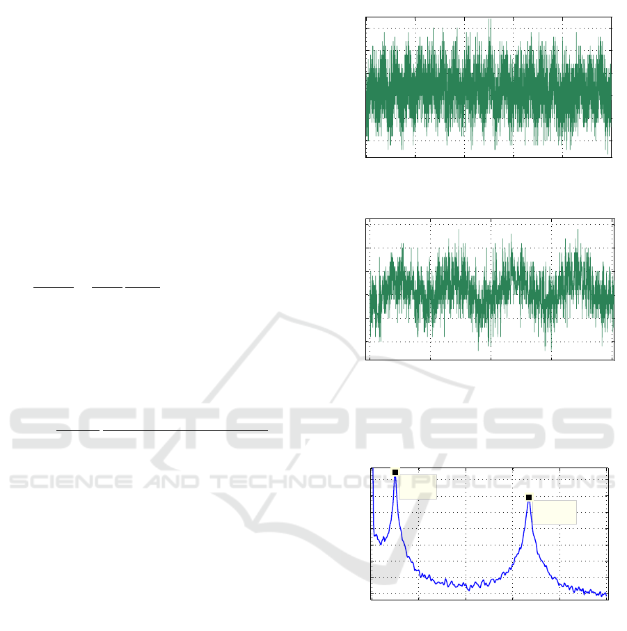
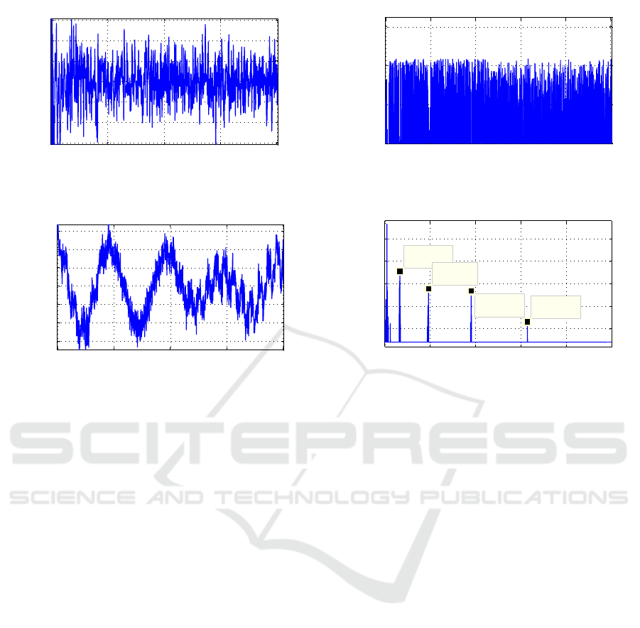
The resonant oscillations of the cantilever, S(t), by
stochastic excitation are shown in Fig. 1. The corre-
sponding PSD obtained as S(ω) = S(ω)S(ω)
∗
is de-
picted in Fig. 2, where S(ω) is FT of S(t). S(t) rep-
resents a signal of a free cantilever, that is, when the
tip of the micro cantilever probe is outside the range
of interfacial force fields, typically a few nanometers
away from the surface.
Practically only few resonances can be directly
observed during the random fluctuations; therefore,
we consider in details only the first and the second
resonance frequencies of the cantilever, i.e., f
(1)
r
=
10 kHz, f
(2)
r
= 66.7 kHz. Nevertheless, the data de-
picted on Fig. 1 allow to analyze much higher res-
onance frequencies because of the total observation
time is t
tot
= 2 ms and a sampling rate is 5 MHz (∆t =
0.2 µs). Obviously, the sampling time ∆t = 0.2 µs
yields an oversampling for the first and for the second
resonances, but it is more suitable for the higher order
resonances.
0 2000 4000 6000 8000 10000
0.07
0.08
0.09
0.1
0.11
0.12
Cantilever output signal, Ts=2.0e-7
Time (Samples)
Amplitude of cantilever,V
0 500 1000 1500 2000
0.07
0.08
0.09
0.1
0.11
0.12
Cantilever output signal, Ts=2.0e-7
Time (Samples)
Amplitude of cantilever,V
Figure 1: Equilibrium state microcantilever output data,
sample time 2 ×10
−7
s a) 10,000 samples, b) 2,000 sam-
ples.
0 2 4 6 8 10
x 10
4
-85
-80
-75
-70
-65
-60
-55
-50
X: 1e+04
Y: -47.73
Fourier Spectrum
Frequency, (Hz)
Spectral density, dBW/Hz
X: 6.7e+04
Y: -55.45
Figure 2: Fourier spectrum of the microcantilever dynamic
response. The peak f
(1)
r
= 10 KHz represents the first res-
onance frequency and at f
(2)
r
= 66.7 KHz represents the
second one.
3 KLT AND ITS DISCRETE
IMPLEMENTATION
3.1 Karhunen-Lo
`
eve Decomposition of
Stochastic Process
One of the simplest and non-expensive orthogonal de-
composition of the stochastic processes from the point
Wireless Sensor Network Microcantilever Data Processing using Principal Component and Correlation Analysis
99

of view of computational complexity is the Fourier
transform (FT) with the complex exponents orthogo-
nal bases functions. Unfortunately, some series draw-
backs of FT, like low resolution of the spectral com-
ponents, slow convergence of the truncated decom-
position to the origin data (especially when the data
vector is short) encourage looking for some other or-
thogonal decompositions techniques with the lack of
mentioned serious weaknesses.
One promising technique that helps to over-
come many drawbacks of Fourier transform is the
Karhunen-Lo
`
eve transform (KLT). KLT is an orthog-
onal transform and it is optimum under the mean
squared error (MSE) between truncated and the ac-
tual data providing the highest convergence of the
data vector into smaller dimension subspace (Lo
`
eve,
1978; Wang, 2012; Marple, 1987). In the opposite
of Fourier transform, where the basis vectors are the
complex exponent functions, the orthogonal basis of
KLT are the eigenvectors of the data covariance ma-
trix. It succeeds very attractive properties, because of
complete decorrelation of the measured data helps to
squeeze the data information into minimum number
of parameters, and, ultimately, among other orthogo-
nal transforms to reach the highest resolution of the
data spectral components (Lo
`
eve, 1978; Wang, 2012;
Marple, 1987).
We propose exploiting the highest resolution
property of KLT applying it for denoising of low Q-
factor cantilever data, thereby significantly increasing
the precision of the resonance frequency estimation.
To introduce KLT we consider a decomposition of
the stochastic data S(t),t ∈ [t
1
,t
2
] as an infinite linear
combination of orthogonal functions in L
2
[t
1
,t
2
]
S(t) =
∞
∑
k=1
Z
k
e
k
(t), (5)
where
Z
k
=
Z
t
2
t
1
S(t)e
k
(t) (6)
are uncorrelated random variables and e
k
(t) is the set
of continuous real-valued functions on [t
1
,t
2
], which
are pairwise orthogonal in L
2
[t
1
,t
2
].
Varying the set of orthogonal functions (6) bearing
the transformations like Fourier transform, wavelet
transform, Haar transform, and so on (Ahmed and
Rao, 1975; Wang, 2012). Kari Karhunen and Michel
Lo
`
eve (Karhunen, 1947; Lo
`
eve, 1978) had found the
set of orthogonal functions that provide the optimum
approximation of the original stochastic process in
the sense of the minimum total mean-square error
[S(t) −
˜
S(t)]
2
, where
˜
S(t) =
∑
L
k=1
Z
k
e
k
(t) is a trun-
cated to L terms decomposition of S(t). The solution
has been found by solving the homogeneous Fred-
holm integral equation of the second kind
Z
t
2
t
1
K
S
(τ,t)e
k
(τ)dτ = λ
k
e
k
(t). (7)
where K
S
(τ,t) the covariance function (kernel) that
satisfies the definition of a Mercer theorem (Wang,
2012) postulating that such a set of eigenvalues λ
k
and
eigenfunctions e
k
(t) exists, which forms an orthonor-
mal basis in L
2
[t
1
,t
2
], and K
S
(τ,t) can be expressed
as
K
S
(τ,t) =
∞
∑
k=1
λ
k
e
k
(τ)e
k
(t). (8)
As a result, (6) becomes the Karhunen Lo
`
eve Trans-
form (KLT), and its basis provide the fastest conver-
gence of
˜
S(t) toward S(t). However, the serious draw-
back of the KLT is the high numerical cost of deter-
mining the eigenvalues and eigenfunctions of its co-
variance operator, because it requires the solution of
the integral equation (7). However, the implementa-
tion of KLT can be significantly simplified when input
data is a discrete random process, because the linear
algebra tools like the eigenvalues decomposition of
discrete covariance matrix can be used. Furthermore,
the fast KLT algorithms can help in some particular
cases (Wang, 2012; Reed and Lan, 1994). Below we
discuss the discrete KLT implementation in details.
3.2 KLT Discrete Implementation
Implementation of discrete KLT is interconnected
with several inconveniences. Firstly, before KLT can
be used for data processing, some preliminary data
preprocessing should be done. It includes, a) storing
in a memory the ”training” set of representative data
samples, b) forming the data covariance matrix, and
c) finding the proper basis functions by computing
the data covariance matrix eigenvalue decomposition.
This preprocessing makes KLT a data dependent lin-
ear transform, and the proper basis functions are never
known a priori excepting when the model of the data
is known. Secondly, KLT has much higher computa-
tional cost and memory requirements that any other
known orthogonal transform restricting both its soft-
ware and hardware implementations. Nevertheless,
KLT is a very attractive tool for data denoising be-
cause of data can be split into two orthogonal sub-
spaces, the useful data and the noisy data, and after-
ward the noisy data can be just ignored. The data de-
noising algorithm that involves KLT includes the fol-
lowing sequence of operations (Wang, 2012).
1. Find the data covariance matrix R =
1
M
∑
M
i=1
S
i
S
T
i
, M ≥ N, where S
i
is a data N ×1
vector, and M is a number of data vector running.
WINSYS 2016 - International Conference on Wireless Networks and Mobile Systems
100

2. Find the eigenvalue decomposition R = ΦΛΦ
T
,
where Λ = [λ
1
,λ
2
,...,λ
N
] is a N × N diagonal
matrix with elements sorted in descending order,
and matrix Φ = [φ
1
,φ
2
,...,φ
N
] is an eigenvectors
matrix, where φ
i
, i = 1, ... ,N, is a N ×1 vectors.
3. Determine the threshold that split the data space
into two subspaces, the subspace of the useful
eigenvalues, and subspace of the unwanted eigen-
values, and determine m significant eigenvalues
which succeed the threshold (m ≤ N).
4. Form N × m truncated KLT transform matrix
Φ
m
= [φ
1
,φ
2
,...,φ
m
] that includes only eigenvec-
tors belonging to larger m eigenvalues of R.
5. Compute direct KLT as y = Φ
T
m
x.
6. Compute inverse KLT as x = Φ
m
y for reconstruc-
tion and data denoising .
Unfortunately, we are not able to practically imple-
ment step 1 because of lack of sufficient statistics –
only one realization of the data vector is available.
To form the full rank matrix R the number of avail-
able realizations must be at least equal to the number
of data points, otherwise the matrix R is a deficient
one. Furthermore, forming the full rank matrix R re-
quires enormous numbers of measurements (at least
10,000 in our case), and posterior tough computa-
tions. However, the computational work can be short-
ened if the true covariance matrix R (it is asymptotical
covariance matrix when M → ∞) can be successfully
replaced by the analytical matrix. Various types of
random processes and their analytical covariance ma-
trices have been derived and presented in (Maccone,
2009). It is well known that in the absence of any ex-
ternal driving forces, the microcantilever accumula-
tive random fluctuations is the Brownian oscillations
process (Mokrane and et al, 2012; Measures, 1984).
Therefore, the analytical Brownian covariance matrix
is formed according to (Maccone, 2009).
4 MICROCANTILEVER DATA
PROCESSING WITH KLT
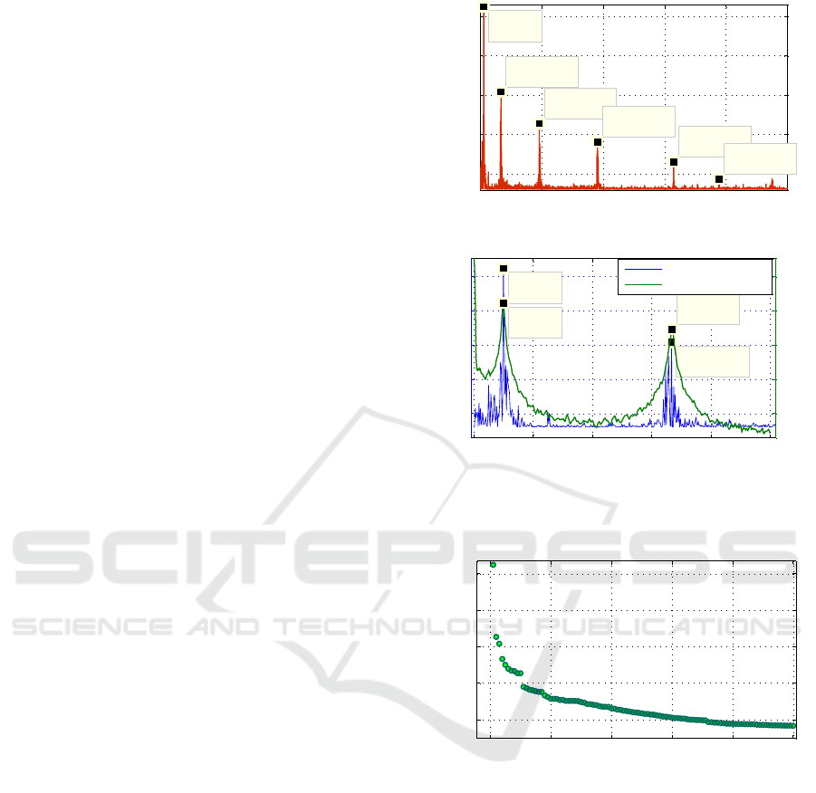
We find the KLT of the data depicted in Fig. 1 using
the algorithm described in Section 3, where all 10,000
eigenvalues are involved. Fig. 3a shows resulting KLT
spectrum for the frequency range 0 - 1 MHz (despite
the whole available range of frequencies for the sam-
ple rate T
s
= 2 ×10
−7
s is 0 - 2.5 MHz), and Fig. 3b
shows KTL spectrum in details in the frequency range
0 - 100 KHz just helping to compare the KLT spec-
trum with the reference FT spectrum.
0 2 4 6 8 10
x 10
5
-25
-20
-15
-10
-5
X: 1e+004
Y: -3.783
KLT Spectrum, (dBW/Hz)
Frequency, (Hz)
X: 6.675e+004
Y: -14.59
X: 1.915e+005
Y: -18.63
X: 3.813e+005
Y: -20.97
X: 6.295e+005
Y: -23.5
X: 7.765e+005
Y: -25.7
0 2 4 6 8 10
x 10
4
-25
-20
-15
-10
-5
X: 1e+004
Y: -3.783
KLT Spectrum, (dBW/Hz)
Frequency, (Hz)
X: 6.675e+004
Y: -14.59
0 2 4 6 8 10
x 10
4
-80
-70
-60
-50
-40
X: 1e+004
Y: -47.73
FT Spectrum, (dBW/Hz)
X: 6.7e+004
Y: -55.45
KLT Spectrum
FFT Spectrum
Figure 3: Cantilever output data Fourier spectrum vs. KLT
spectrum a) f
max
= 1 MHz, b) f
max
= 100 kHz.
0 20 40 60 80 100
-25
-20
-15
-10
-5
Eigenvalues distribution
Eigenvalue #
Eigenvalues intensity (V)
Figure 4: Distribution of the first 100 eigenvalues of data.
As follows from Fig. 3 the KLT spectrum has
much higher resolution than the reference FT spec-
trum, even in the presence of complementary noise
that can both distort and displace the result of reso-
nance peak frequencies measurements. However, de-
noising of the original data helps to identify the res-
onance frequencies with more higher precision. We
start the data denoising with finding of the data co-
variance matrix eigenvalues distribution, and the re-
sult is presented in Fig. 4. Applying the KLT to the
output data and afterward reconstructing the data in-
volving the very first largest eigenvalue resulting the
perfect emerging of high resolved peak on the first
resonance frequency 10 kHz. Then involving three
largest eigenvalues results the second peak at the fre-
Wireless Sensor Network Microcantilever Data Processing using Principal Component and Correlation Analysis
101

0 2 4 6 8 10
x 10
4
-100
-80
-60
-40
-20
0
X: 1e+04
Y: -6.779
Frequency, (Hz)
Spectral density, dBW/Hz
X: 6.675e+04
Y: -17.41
FT Spectrum
KLT Spectrum
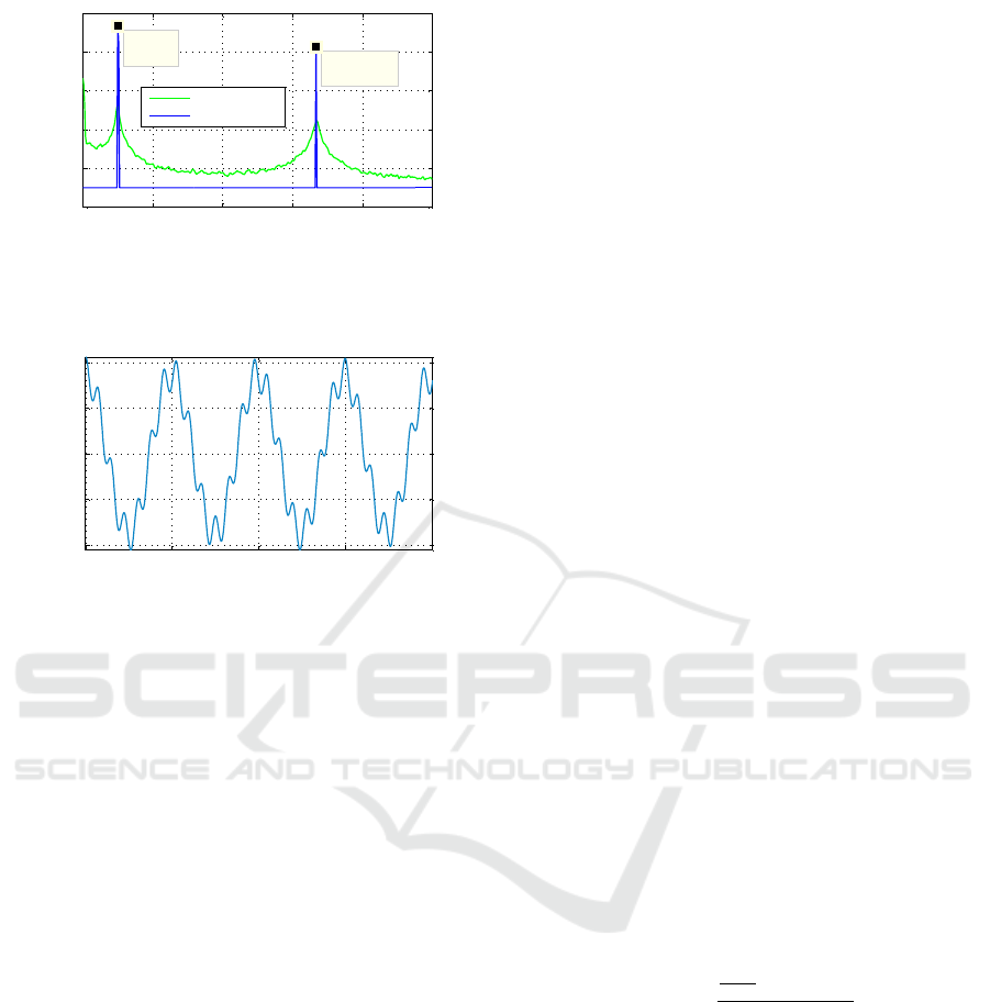
Figure 5: Estimation of the first and the second resonance
frequency peaks involving three largest eigenvalues.
0 500 1000 1500 2000
-0.01
-0.005
0
0.005
0.01
Output data, descarding three largest eigenvalues out of 10,000
Time (Samples)
Amplitude of cantilever,V
Figure 6: Data reconstructed using three largest eigenval-
ues.
quency 66.7 kHz as Fig. 5 shows. Emerging strong
and narrow peaks helps to estimate resonance fre-
quencies with much higher precision than those that
can be provided by the reference spectrum obtained
by FT. Fig. 6 depicts the time domain data when the
first three eigenvalues are used in computing of the in-
verse KLT , where the first and the second resonance
frequencies can be recognized as the lower and the
higher frequencies oscillated waves, respectively.
5 THRESHOLD
DETERMINATION BETWEEN
USEFUL PATTERN AND NOISE
USING CORRELATION
ANALYSIS
In previous section to detect and identify the res-
onance frequencies we involve the fist three larger
eigenvalues that correspond to the first and to the sec-
ond resonances, e.i., 10.0 kHz and 66.7 kHz, and
the rest of the eigenvalues were discarded as un-
wanted. However, as Fig. 3a shows, KLT spectrum
allows to estimate the higher order resonance frequen-
cies as well. Particularly, 191.5 kHz, 381.3 kHz,
629.5 kHz and 776.5 kHz, which can provide ad-
ditional meaningful information about the measured
data. It means that all eigenvalues that represent the
higher order resonance frequencies belong to the set
of eigenvalues that bearing additional useful informa-
tion. Hence, discrimination of the desire eigenvalues,
which represent the useful data and unwanted eigen-
values which represent the purely stochastic com-
ponents, refers to the threshold determination prob-
lem. Finding appropriate threshold helps to solve
the data denoising problem, i.e., to suppress the in-
terfering random fluctuations that distort the reso-
nance frequencies measurement result. The thresh-
old determination problem is formulated as following
(Marple, 1987). In the whole set of N eigenvalues
Λ = {λ
1
,λ
2
,...,λ
m
,λ
m+1
,...,λ
N
}obtained by eigen-
values decomposition of the data covariance matrix
determine the value m, 1 < m < N, that splits the set Λ
into two orthogonal subspaces, one of them is a signal
subspace, Λ
S
, that contains the useful deterministic
components (excited the resonances) and other one,
Λ
n
, is a subspace of the random noise that contains
uncorrelated residual components (interferer), i.e.
R =
m
∑
k=1
λ
k
φ
k
φ
H
k
+
N
∑
k=m+1
λ
k
φ
k
φ
H
k
, (9)
where unknown value m must be determined. In the
literature numerous attempts are done to determine
the value m. For example, Konstantinides (Konstan-
tinides and Yao, 1988) propose firstly to find the ratio
(
∑
m
k=1
λ
k
/
∑
N
k=1
λ
k
)
1/2
, and then compare it with some
predetermined value ε, which depends on the vari-
ance of the random noise; however it require a priory
information about the variance of the noise, hence,
some additional measurements or analysis of data is
needed. Marple (Marple, 1987) propose to use the
rule based on the Akaike information criterion (AIC)
(Sakamoto et al., 1986), that is
AIC{m}= (N −m)ln(
1
N−m
∑
m
k=m+1
λ
k
∏
m
k=m+1
λ
N−m
k
)+m(2N −m).
(10)
Afterward, the minimum AIC over all m should be
chosen. Despite the Akaike criteria estimates a rela-
tive information lost for a given data model, it does
not provide the testing of a null hypothesis, meaning
that some weak amplitude components of a useful sig-
nal can be lost.
Below we propose the solution of the threshold es-
timation problem by using the correlation analysis of
the stochastic data subspace in order to find the subset
that contains only the random uncorrelated compo-
nents. Other words, we find the value m using the trial
and errors approach ensuring that
∑
N
k=m+1
λ
k
φ
k
φ
H
k
is a
random uncorrelated data. For this, we successively
WINSYS 2016 - International Conference on Wireless Networks and Mobile Systems
102

-1 -0.5 0 0.5 1
x 10
4
0
0.2
0.4
0.6
0.8
1
Autocovariance after descarding three largest eigenvalues
Lag
Coefficients
-1 -0.5 0 0.5 1
x 10
4
0
0.2
0.4
0.6
0.8
1
Autocovariance after descarding three largest eigenvalues
Lag
Coefficients
-1 -0.5 0 0.5 1
x 10
4
-0.2
0
0.2
0.4
0.6
0.8
1
Autocovariance after descarding 50 largest eigenvalues
Lag
Coefficients
-1 -0.5 0 0.5 1
x 10
4
0
0.2
0.4
0.6
0.8
1
Autocovariance after descarding 110 largest eigenvalues
Lag
Coefficients
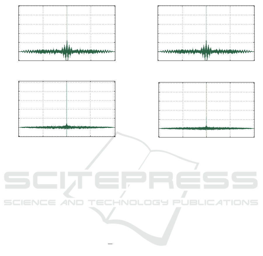
Figure 7: Data autocovariance after a) discarding three larger eigenvalues, b) discarding 20 larger eigenvalues, c) discarding
50 larger eigenvalues, d) discarding 110 larger eigenvalues.
discard m = 1,2,..., N larger eigenvalues from the
data and for each m we are testing the null hypoth-
esis of the rest of the data. The resulting autoco-
variance function when m is 3, 20, 50 and 110 are
presented in Fig. 7. As follows from Fig. 7, when
only 3 or even 20 largest eigenvalues are discarded,
the correlation is still high (lagged correlation coeffi-
cients oscillat with the high amplitudes), but when the
number of largest eigenvalues to be discarded are in-
creasing, then lagged correlation coefficients are get-
ting lower approaching the level −N ±2/
√
N, and
for m = 110 the null hypothesis (the sequence rep-
resents the random process with zero correlation) can
be accepted inside the 95% confidence interval lim-
its (Kendall et al., 1977). Resulting plots of splitting
random noise and deterministic pattern when m = 110
in both time and frequency domains are depicted in
Fig. 8, and Fig. 9, respectively. Visually Fig. 8 repre-
sents the poorly random data showing stochastic fluc-
tuation in the time domain and almost equal ampli-
tudes of all eigenvalues in the frequency domain (con-
sist with PSD of the random noise), and Fig. 9 repre-
sents deterministic data, showing predicted behavior
in the time domain and expressive peaks on the fre-
quency domain (consist with deterministic pattern be-
havior). It just confirms that after the null hypothesis
testing the determined threshold is found correctly.
6 CONCLUSIONS
We present and analyze microcantilever data denois-
ing technique using one of the more advanced orthog-
onal transforms – Karhunen-Lo
`
eve Transform (KLT),
which helps to split the eigenvalue decomposition of
measured data covariance matrix by two independent
subsets – subset of useful signal that contains the
larger eigenvalues, and subset of unwanted signal that
contains the rest of eigenvalues. Processing of data
with the first three larger eigenvalues and discarding
the rest of them we perfectly determined the first and
second resonance frequencies of the microcantilever
with high precision.
We proposed to use the correlation analysis and
the null hypothesis testing to determine the optimum
threshold between subsets of deterministic eigenval-
ues and eigenvalues that belong to the random fluctu-
ations. The simulation result confirm the truthful of
proposed approach.
The KLT has been demonstrated the ability of ef-
fective improvement of the spectral identification of
the micro cantilever resonances that were driven by
the Brownian noise (thermal, mechanical, electronic
and other type of random fluctuations). The simula-
tion results and analytical analysis illustrate that KLT
can be adapted as a powerful data denoising tool for
the cantilever based sensing applications.
Wireless Sensor Network Microcantilever Data Processing using Principal Component and Correlation Analysis
103

0 500 1000 1500 2000
-6
-4
-2
0
2
4
6
x 10
-5
Residual data, discarding 110 largest eigenvalues
Time (Samples)
Amplitude of noise,V
0 2 4 6 8 10
x 10
5
-50
-45
-40
-35
Frequency, (Hz)
Noise spectral density, dBW/Hz
KLT of resifual data
Figure 8: Residual noise after discarding of 110 larger eigenvalues a) time domain, b) frequency domain.
0 500 1000 1500 2000
-0.015
-0.01
-0.005
0
0.005
0.01
0.015
Output data, including 109 largest eigenvalues out of 10,000
Time (Samples)
Amplitude of cantilever,V
0 2 4 6 8 10
x 10
5
-30
-25
-20
-15
-10
X: 6.675e+04
Y: -17.29
Frequency, (Hz)
Spectral density, dBW/Hz
KLT of 109 largest eigenvalues out of 10,000
X: 1.93e+05
Y: -21.11
X: 3.813e+05
Y: -21.66
X: 6.295e+05
Y: -28.51
Figure 9: Deterministic pattern involving 109 larger eigenvalues a) time domain, b) frequency domain.
ACKNOWLEDGEMENTS
This work was supported by the laboratory directed
research and development (LDRD) fund at Oak Ridge
National Laboratory (ORNL). Viktor Zaharov ac-
knowledges the financial support received from the
Department of Energy (DOE) Visiting Faculty Pro-
gram (VFP). ORNL is managed by UT-Battelle,
LLC, for the US DOE under contract DE-AC05-
00OR22725.
REFERENCES
Ahmed, N. and Rao, K. (1975). Orthogonal transforms for
digital signal processing. Springer-Verlag.
Albrecht, T. R., Grtitter, P., Horne, D., and Rugar, D.
(1991). Frequency modulation detection using highd-
kantilevers for enhanced force microscope sensitivity.
J. Appl. Phys., 69(2).
Bengtsson, M., Gr
¨
onlund, R., Lundqvist, M., Larsson, A.,
Kr
¨
oll, S., and Svanberg, S. (2006). Remote laser-
induced breakdown spectroscopy for the detection and
removal of salt on metal and polymeric surfaces. Ap-
plied Spectroscopy, 60:1188–1191.
Buchapudi, K. R., Huang, X., Yang, X., Ji, H. F., and Thun-
dat, T. (2011). Microcantilever biosensors for chemi-
cals and bioorganisms. Analyst, (136(8)):1539–1556.
Dada, O. O. and Bialkowski, S. E. (2011). A compact,
pulsed infrared laser-excited photothermal deflection
spectrometer. Applied Spectroscopy, 65(2):201–205.
Farahi, R. H., Passian, A., Jones, Y. K., Tetard, L., Lereu,
A. L., and Thundat, T. G. (2012). Pumpprobe pho-
tothermal spectroscopy using quantum cascade lasers.
Journal of Physics D, 45:125101.
Karhunen, K. (1947).
¨
Uber lineare methoden in der
wahrscheinlichkeitsrechnung. Ann. Acad. Sci. Fen-
nicae, Ann. Acad. Sci. Fennicae. Ser. A. I. Math.-
Phys.(37):1–79.
Kawakatsu, H., Kawai, S., Saya, D., Nagashio, M.,
Kobayashi, D., Toshiyoshi, H., and Fujita, H. (2002).
Towards atomic force microscopy up to 100 MHz. Re-
view of Scientific Instrument, 73(2317).
Kendall, M. G., Stuart, A., and Ord, J. K. (1977). The ad-
vanced theory of statistic. Griffin.
Konstantinides, K. and Yao, K. (1988). Statistical analysis
of effective singular values in matrix rank determina-
tion. Acoustics, Speech and Signal Processing, IEEE
Transactions on, 36(5):757 – 763.
Labuda, A., Bates, J. R., and Gr
¨
utter, P. H. (2012). The noise
of coated cantilevers. Nanotechnology, 23(025503).
Lo
`
eve, M. (1978). Probability theory. Graduate Texts in
Mathematics, volume 2. Springer-Verlag, 4th edition.
Lozano, J. and Garcia, R. (2009). Theory of multifrequency
atomic force microscopy. Phys. Rev. B, 79(014110).
Maccone, C. (2009). Deep Space Flight And Communica-
tion. Springer.
WINSYS 2016 - International Conference on Wireless Networks and Mobile Systems
104

Marple, S. L. (1987). Digital Spectral Analysis with Appli-
cation. Prentice-Hal.
Measures, R. M. (1984). Laser Remote Sensing: Funda-
mentals and Applications. Wiley-Interscience.
Mokrane, B. and et al (2012). Study of thermal and acous-
tic noise interferences in low stiffness atomic force
microscope cantilevers and characterization of their
dynamic properties. Review of Scientific Instruments,
83(1).
Parmeter, J. E., editor (2004). The challenge of standoff
explosives detection. 0-7803-8506-3/02. IEEE.
Passian, A., Lereu, A. L., Yi, D., Barhen, S., and Thun-
dat, T. (2007). Stochastic excitation and delayed os-
cillation of a micro-oscillator. Physical Review B,
75:233403.
Reed, I. S. and Lan, L.-S. (1994). A fast approximate
karhunen-lo
`
eve transform (aklt) for data compression.
Journal of Visual Communication and Image Repre-
sentation, 5:304–316.
Sakamoto, Y., Ishiguro, M., and Kitagawa, G. (1986).
Akaike Information Criterion Statistics. Springer.
Van Neste, C. W., Senesac, L. R., and Thundat, T. (2009).
Standoff spectroscopy of surface adsorbed chemicals.
Analytical Chemistry, 81(5):1952–1956.
Wang, R. (2012). Introduction to Orthogonal Transforms:
With Applications in Data Processing and Analysis.
Cambridge University Press.
Wig, A., Arakawa, E. T., Passian, A., Ferrell, T. L., and
Thundat, T. (2006). Photothermal spectroscopy of
bacillus anthracis and bacillus cereus with microcan-
tilevers. Sensors and Actuators B, 114:206.
Wireless Sensor Network Microcantilever Data Processing using Principal Component and Correlation Analysis
105