Inferring Causality from Noisy Time Series Data

A Test of Convergent Cross-Mapping

Dan Mønster

1,2,∗

, Riccardo Fusaroli

2,3

, Kristian Tyl

3,2

, Andreas Roepstorff

and Jacob F. Sherson

4,5

Department of Economics and Business Economics, Aarhus University, Fulglesangs All

e 4, 8210 Aarhus V, Denmark

Interacting Minds Centre, Aarhus University, Jens Chr. Skous Vej 4, 8000 Aarhus C, Denmark

Center for Semiotics, Aarhus University, Jens Chr. Skous Vej 2, 8000 Aarhus C, Denmark

Department of Physics and Astronomy, Aarhus University, Ny Munkegade 120, 8000 Aarhus C, Denmark

AU Ideas Center for Community Driven Research, Aarhus University, Ny Munkegade 120, 8000 Aarhus C, Denmark

Keywords:

Convergent Cross-Mapping, Causality, Logistic Map, Noise, Time Series Analysis.

Abstract:

Convergent Cross-Mapping (CCM) has shown high potential to perform causal inference in the absence of

models. We assess the strengths and weaknesses of the method by varying coupling strength and noise levels in

coupled logistic maps. We ﬁnd that CCM fails to infer accurate coupling strength and even causality direction

in synchronized time-series and in the presence of intermediate coupling. We ﬁnd that the presence of noise

deterministically reduces the level of cross-mapping ﬁdelity, while the convergence rate exhibits higher levels

of robustness. Finally, we propose that controlled noise injections in intermediate-to-strongly coupled systems

could enable more accurate causal inferences. Given the inherent noisy nature of real-world systems, our

ﬁndings enable a more accurate evaluation of CCM applicability and advance suggestions on how to overcome

its weaknesses.

1 INTRODUCTION

The ability to infer causality from the relation between

two variables is an intensely researched area. Com-

mon approaches involve having both a model of the

system being studied and a series of measurements

of that same system (Pearl, 2009). In many cases,

however, we do not have an adequate model of the

system, or face several conﬂicting models. Complex

natural, technical and social systems are prime exam-

ples, including ecosystems, brains, the climate and

the global ﬁnancial system. In such cases, inferring

whether one part has a causal inﬂuence on another part

has to rely on model-free methods. Convergent Cross-

Mapping (CCM) (Sugihara et al., 2012) is a relatively

new method that promises to ‘distinguish causality

from correlation’ in time series data (ibid., p. 496).

CCM was introduced as an alternative to other meth-

ods that detect causality between two time series, prin-

cipally Granger causality (Granger, 1969).

Granger causality has been developed to assess eas-

ily separable linear systems, whereas CCM is primarily

suited for weakly coupled components of non-linear

dynamic systems. Accordingly, they have slightly di-

verging notions of causality. Therefore, the statement

‘

causes

’ would more accurately be phrased as ‘

Granger causes

’ or ‘

CCM causes

’. Sugihara

et al. (2012) refer to the type of causality captured

by CCM as dynamic causation, reminiscent of what

Lakoff (2010) terms systemic causation. For a system

with several variables, for which time series data are

available, the CCM method produces a causal network

structure describing which variables are causally con-

nected, including the direction of causality. Like mu-

tual information (Fraser and Swinney, 1986), transfer

entropy (Schreiber, 2000) and cross-recurrence quan-

tiﬁcation (Webber and Zbilut, 1994; Marwan et al.,

2007) CCM is a state space method relying on time-

delayed embedding of the time series data in a higher

dimensional space.

CCM has already been used in a wide range of

different ﬁelds for different kinds of data (McBride

et al., 2015; BozorgMagham et al., 2015; McCracken

and Weigel, 2014), and it has been noted (McCracken

and Weigel, 2014) that CCM results are not always

consistent with theoretical intuitions. McCracken and

Weigel (2014) extended CCM to pairwise asymmetric

inference (PAI), which they demonstrated to give re-

sults that are in better accordance with the intuitively

expected outcomes for several physical systems. Re-

Mønster, D., Fusaroli, R., Tylén, K., Roepstorff, A. and Sherson, J.

Inferring Causality from Noisy Time Series Data - A Test of Convergent Cross-Mapping.

In Proceedings of the 1st International Conference on Complex Information Systems (COMPLEXIS 2016), pages 48-56

ISBN: 978-989-758-181-6

cently Ma et al. (2014) developed cross-map smooth-

ness (CMS)—a method related to CCM—which has

the advantage of requiring fewer points in the time

series. Notice, however, that in this paper we focus on

CCM, leaving the analysis of developments such as

PAI and CMS for future work.

Given the interest and relevance of CCM, it is im-

portant to better understand its strengths and limita-

tions. Accordingly, in this article we will present re-

sults of an in-depth study of a simple model system,

the coupled logistic map, with particular emphasis on

how the CCM results reﬂect the model input, vary-

ing strength of coupling, and levels of noise. We will

brieﬂy describe how CCM is applied to the model.

Then we look at how the choice of coupling affects the

CCM results, and ﬁnally we report on results of adding

noise to the system. Although noise in real-world data

is ubiquitous, the inclusion of noise in model investiga-

tions has been largely neglected. We ﬁnd that noise can

dramatically change the strength of causal inferences.

Crucially, we also observe that the appropriate injec-

tion of noise into the dynamics can be used as means

of inferring the relative strengths of the coupling (to

the extent that the system can be controlled).

2 MODEL SYSTEM

The logistic map has long been a model system of non-

linear dynamics displaying regular periodic behavior

as well as deterministic chaos (May, 1976). A sys-

tem of two coupled logistic maps has been used as a

simple model of chemical reaction dynamics (Ferretti

and Rahman, 1988) and population dynamics (Lloyd,

1995). This makes it an ideal model system for testing

CCM. We follow Sugihara et al. (2012) and study two

logistic maps coupled through linear terms

t+1

= x

(1 − x

) − β

)

t+1

= y

(1 − y

) − β

)

(1)

The two variables

and

have a nonlinear de-

pendence on their own past values parameterized by

the growth rates

, and are coupled to each other

through linear terms with coupling constants that pa-

rameterize the strength of the coupling from

(β

)

and from

x (β

)

. Times series for

and

are shown in Figure 1 for a particular choice of the

parameters in the model.

A single logistic map has well-known domains

of periodic behavior controlled by the growth rate

. As

becomes larger, increasingly frequent period-

doublings occur, which ultimately give way to chaotic

behavior at

r ≈ 3.57

. This well-known phase diagram

300 305 310 315 320 325 330

0.2

0.3

0.4

0.5

0.6

0.7

0.8

0.9

, y

Figure 1: Plot of the time series of

(shown in blue) and

(shown in red) after the initial 300 time steps. Note that

= 0

, so there is no coupling from

and the causality

is therefore unidirectional from

y (β

= 0.05)

. Both

= 3.65

and

= 3.77

are chosen to be in a chaotic regime

of the logistic map.

or bifurcation diagram is shown in the bottom panel

of Figure 2, representing the

variable. The top panel

shows the phase diagram for another logistic map rep-

resenting the

variable. In order to illustrate the effect

of coupling between two logistic maps the growth rate

for the

variable

is related to

by the equation

+ r

= 6.5

. This is the equation for a line in the

)

-plane with a slope of

−1

. The middle panel

in Figure 2 illustrates the phase diagram of

for a

family of two coupled logistic maps along this line in

the

)

-plane as described by Eq. 1 with

= 0

and β

= 0.2.

The middle and lower panels show the effect of

unidirectional coupling between two logistic maps. It

is evident that the dynamics of

leaves an imprint on

as indicated by the ﬁxed points. For low

(high

) where the isolated system (top panel) is stationary,

the effect of coupling from the chaotic dynamics of

induces chaotic dynamics in

, albeit with a much

smaller amplitude. For high

(low

) where the iso-

lated system is chaotic, the coupling from

which is

in the stationary domain has the effect of stabilizing

the periodic phases of

which persist to higher values

of r

than in the isolated system.

2.1 Noise

Real-world systems present varying degrees of envi-

ronmental and measurement noise and the application

of the method to such systems thus critically depends

on the method’s ability to cope with noise. We there-

fore also consider the model with added noise terms:

t+1

= x

(1 − x

) − β

) + ε

x,t

t+1

= y

(1 − y

) − β

) + ε

y,t

(2)

Inferring Causality from Noisy Time Series Data - A Test of Convergent Cross-Mapping

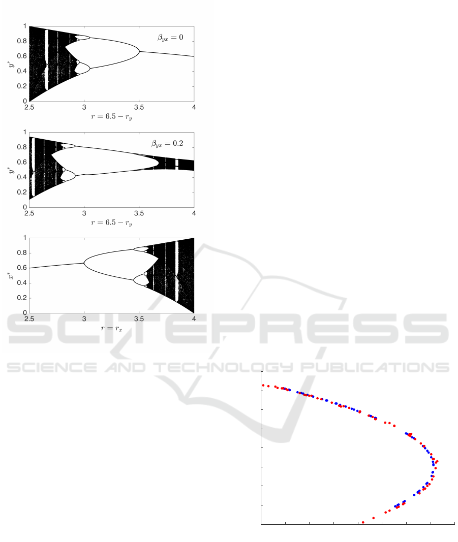
Figure 2: Phase diagram for the coupled logistic map in Eq. 1

for

= 0

. The growth rates

are parameterized by the

variable

on the horizontal axis as

= r

and

= 6.5 − r

For each value of

the plots represent a different pair of

parameters

. The bottom panel shows the ﬁxed points

∗

as a function of the growth rate, and the top panel

(β

= 0)

shows the ﬁxed points

∗

. The center panel shows the ﬁxed

points for β

= 0.2.

Here

x,t

and

y,t

are the noise terms on

and

which we model as stochastic variables sampled from

normal distributions

N (0, σ

)

with zero mean and

standard deviation

. We will refer to

as the noise

level. Note that noise in either variable in Eq. 2 prop-

agates to later values of the variable and to the other

variable through the coupling terms. Hence, the noise

terms in this model represent perturbations from the

environment rather than noise from the measurement

process.

3 METHOD

Convergent cross-mapping is a state space method

that relies on Takens’ theorem (Takens, 1981) to re-

construct the underlying dynamics of a system in a

model-free fashion, by using time-delayed embed-

ding to reconstruct its attractor landscape (see, e.g.,

Abarbanel (1996)). Our model system in Eq. 1 can

be described by its attractor, that is, the trajectory

consisting of consecutive points in two-dimensional

Euclidean space given by the Cartesian coordinates

),(x

),...,(x

)

resulting from the dy-

namics described by Eq. 1. We discard the ﬁrst 300

points to avoid transient behavior of the model from

affecting our results. According to Takens’ theorem

we can approximately reconstruct the attractor from

one of the variables

alone using time-delayed

embedding of the points in one of the time series, say

, where each point in

-dimensional space is given

= (x

t−τ

t−2τ

,...x

t−(E−1)τ

)

. The embedding

thus depends on two parameters: the time delay

and the dimension

of the space in which the recon-

structed attractor is embedded. Since we know that

there are only two independent variables in our model

system we choose

E = 2

, but estimating the embed-

ding dimension from the times series obtained from

Eq. 1 using the false nearest neighbor method (Abar-

banel, 1996) gives the same result. The time delay

for the embedding was set to

τ = 1

based on the aver-

age mutual information criterion (Kantz and Schreiber,

1997). The reconstructed attractors, referred to as

shadow manifolds by Sugihara et al. (2012), are shown

in Figure 3.

The two key ingredients of the CCM method are

the concept of cross-mapping and the convergence

property that are explained in the following sections.

0.2 0.3 0.4 0.5 0.6 0.7 0.8 0.9 1

, y

0.2

0.3

0.4

0.5

0.6

0.7

0.8

0.9

t−1

, y

t−1

Figure 3: The shadow manifolds based on the time series

displayed in Figure 1, embedded using

E = 2

and

τ = 1

. A

total of 60 points

= (x

t−1

)

are shown in blue and

the points y

= (y

t−1

) in M

are shown in red.

3.1 Cross-mapping

The time series data from each variable—in our case

and

—can be used to construct shadow manifolds—

COMPLEXIS 2016 - 1st International Conference on Complex Information Systems

and

—that are approximations to the true attrac-

tor. Given the non-separability of the system, Taken’s

theorem demonstrates that when two different vari-

ables represent different parts of the same dynamical

system their shadow manifolds are diffeomorphic to

the true attractor and therefore to each other. Intu-

itively the two variables are connected because they

are part of the same dynamical system as evidenced

by the fact that they both represent a dimension in

the state space. So, if

has a causal inﬂuence on the

dynamics of

then

will inﬂuence the dynamics of

This ‘imprint’ of

means that knowledge of the

shadow manifold M

obtained from the time series of

can be used to estimate values of

. This estimate is

called the cross-map and is denoted ˆx|M

To ﬁnd the cross-mapped estimate

ˆx

start by identifying the corresponding point

Since

is diffeomorphic to

, a small region around

will map to a small region around

and this can

be used to estimate

. To form a bounding simplex

around

at least

E + 1

points are needed (Sugihara

and May, 1990), so the

E + 1

nearest neighbors of

are found. Sorted from the closest to the farthest

point from

we call these

,...,y

E+1

. We use

the points in the time series for

at the corresponding

times, i.e., x

,...,x

E+1

to estimate x

ˆx

E+1

∑

i=1

(3)

The weights

are exponentially weighted with the

Euclidean distance between

and the nearest neigh-

bor points:

= u



E+1

∑

j=1

, u

= exp



−

− y



(4)

where

is the Euclidean norm in R

Estimating one point alone is not sufﬁcient to show

how well

ˆx

estimates the true value

. A library

consisting of

points from

is therefore used to

provide estimates of

points in the time series for

The Pearson correlation coefﬁcient ρ

x ˆx

between the L

true values from

and the

cross-mapped estimates is

an indicator of how much the dynamics of

inﬂuences

the dynamics of

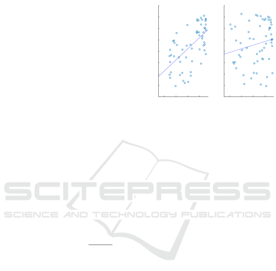
. Scatter plots of observed values

and cross-mapped estimates of

and

are shown in

Figure 4.

The results indicate that the cross-mapped esti-

mates of

obtained from

(ρ

x ˆx

≈ 0.6)

are better

than the cross-mapped estimates of

obtained from

(ρ

y ˆy

≈ 0.2)

. It is therefore tempting to conclude

that

causes

, but, although correct in this case, such a

conclusion is potentially misleading. Indeed, A slight

variation in the parameters, can produce results that

0.2 0.4 0.6 0.8

0.2

0.3

0.4

0.5

0.6

0.7

0.8

0.9

ˆx|M

x,ˆx

= 0.6

0.2 0.4 0.6 0.8

0.2

0.3

0.4

0.5

0.6

0.7

0.8

0.9

ˆy|M

y,ˆy

= 0.19

Figure 4: Scatter plot of pairs of observed values of

and

estimated values

ˆx|M

(left panel) and the equivalent for

(right panel). The cross-mapped estimates were computed

according to Eq. 3 and were based on the shadow manifolds

in Figure 3.

would lead to the opposite conclusion. The additional

criterion of convergence is crucial to correctly infer

the direction and relative strength of causality.

Cross-mappings were performed with XMAP

(Mønster, 2013) which was developed in MATLAB

and validated by reproducing the results by Sugihara

et al. (2012) and by comparing with an independently

developed algorithm (Jespersen, 2013). A small reg-

ularizing term

is added to the denominator in the

argument to the exponential function in Eq. 4 in or-

der to avoid ﬂoating point overﬂow in cases where

= y

3.2 Convergence

The convergence properties of the correlation between

observed values and cross-mapped estimates as a func-

tion of the library length

is the second key ingredient

in CCM. If

causes

then the estimate of

obtained

from

should improve as the number of points

sampled from

becomes larger, since the library of

samples will become a better and better representation

of the attractor, and the nearest neighbor points will be

closer and closer to y

This convergence phenomenon is illustrated in Fig-

ure 5 where correlations derived from the data shown

in Figure 4 have been computed for increasing values

of the library length. Figure 5 shows that

x ˆx

converges

toward a much higher value than

y ˆy

does. This is evi-

dence that

enables much better estimates for

than

does for

. Note that cross-mapped estimation skill

is from y to x when x causes y.

Inferring Causality from Noisy Time Series Data - A Test of Convergent Cross-Mapping

0 50 100 150 200 250 300 350 400

-0.3

-0.2

-0.1

0.1

0.2

0.3

0.4

0.5

0.6

0.7

Figure 5: The correlation coefﬁcient

x, ˆx

(blue circles) and

y, ˆy

(red circles) as a function of library length

. Fits to

the function in Eq. 5 are shown as solid lines. For

the

converged value is

∞

= 0.71

, and for

it is

∞

= 0.096

Parameter values:

= 3.65

= 3.77

= 0

= 0.05

3.2.1 Fitting the Convergence

Rather than relying only on the value of the correlation

coefﬁcient for the largest obtained value of

we ﬁt

the computed values of

as a function of

to the

following function

ρ(L) = αe

−γL

+ ρ

∞

. (5)

This function, containing three constants

and

∞

is in accordance with the computed values of the corre-

lation coefﬁcient. It can be interpreted as convergence

toward the value

∞

L → ∞

where the speed of con-

vergence is given by the constant

. The third constant

is necessary to obtain a good ﬁt, but does not provide

additional interpretive value.

The solid lines in Figure 5 represent the ﬁtted cor-

relation coefﬁcients to the function in Eq. 5 using the

same parameters as in Figure 1. The ﬁtted value for

x ˆx

∞

= 0.71 ±0.046

(95% CI), and the ﬁtted value

for ρ

y ˆy

is ρ

∞

= 0.096 ± 0.024.

4 RESULTS

The previous section introduced CCM and demon-

strated how to apply the method on the model system

using a particular choice of parameter values as an ex-

ample. Sugihara et al. (2012) summarize their results

for different values of the coupling constants

and

with

and

chosen uniformly from the interval

[3.6,4]

in Figure 3B of their manuscript. This ﬁgure

indicates that CCM gets the direction of the coupling

right, but also indicates that for some choices of the

coupling constants the method may give results that

100 200 300

0.2

0.4

0.6

0.8

= 0.1

100 200 300

0.2

0.4

0.6

0.8

= 0.2

100 200 300

0.2

0.4

0.6

0.8

= 0.5

100 200 300

0.2

0.4

0.6

0.8

= 2

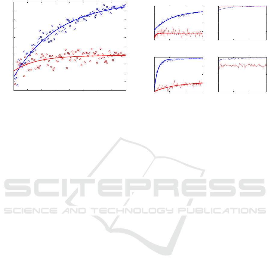
Figure 6: Correlations between observed and cross-mapped

estimates of

(blue) and

(red) for four different values of

. Thin lines are the computed correlations and thick lines

are ﬁts to Eq. 5. For

= 0.2

and

= 2

a good ﬁt is not

possible, and no ﬁts are shown.

are hard to distinguish from symmetric coupling, even

when β

 β

or vice versa.

To investigate this further, we will look at what

happens for a particular choice of

and

when the

coupling between the two variables is manipulated.

4.1 Effect of Weak and Strong Coupling

To study how CCM causality estimates depend on the

strength of the coupling between the two variables we

ﬁx

= 3.625

and

= 3.77

. To keep things simple,

we will set

= 0

as in the previous example, and

only vary

. The correlation coefﬁcients

x ˆx

and

y ˆy

are shown in Figure 6 for β

= 0.1, 0.2, 0.5, 2.0.

For

= 0.05

, a plot very similar to that displayed

in Figure 5 is produced (not shown in Figure 6), which

is consistent with a coupling from

, but no cou-

pling from y to x.

For

= 0.1

x, ˆx

is seen to converge toward

∞

0.89

, whereas

y, ˆy

ﬂuctuates around 0.36. This lack

of convergence as a function of the library size is an

indication that there is no coupling from y to x.

For

= 0.5

, the convergence of

x ˆx

is toward

the higher value

∞

= 0.96

, and convergence is faster,

indicating a stronger coupling. Here we also see con-

vergence of

y ˆy

toward

∞

= 0.43

, and although the

value is much smaller than for

, this could indicate a

coupling from

. We know that this is not the case,

since

= 0

, so instead this is most likely due to the

fact that

is driving

, and that the two time series are

becoming more synchronized.

For an intermediate

value of 0.2 something

unexpected happens: both

x ˆx

and

y ˆy

quickly increase

to values close to 1, already for very low values of

COMPLEXIS 2016 - 1st International Conference on Complex Information Systems

. Furthermore for

L . 100

y ˆy

> ρ

x ˆx

. Naively this

could be seen as an indication that there is a strong

bidirectional coupling between

and

. Alternatively

both signals could be driven by a common external

variable—the Moran effect (Moran, 1953)—or one of

the variables is driving the other so strongly that they

synchronize (Boccaletti et al., 2002; Pikovsky et al.,

2003). We know, however, that neither the Moran

effect, nor synchronization can be the explanation here,

so a different explanation must be found. We return to

this in section 4.1.1, but note here that (i) for both

and

the correlation is uniformly high, i.e., there is not

much evidence of convergence, and (ii) the function in

Eq. 5 is not a good ﬁt to the data.

For

= 2

we again see very high correlation

coefﬁcients for both

and

, but clearly

x ˆx

> ρ

y ˆy

There is not much evidence of convergence for

x ˆx

and

y ˆy

ﬂuctuates around a value close to 0.8. This

is consistent with synchronization due to the strong

coupling from

and inspection of the time series

conﬁrms this. Again we note that

ρ(L)

from Eq. 5 is

not a good ﬁt to the data.

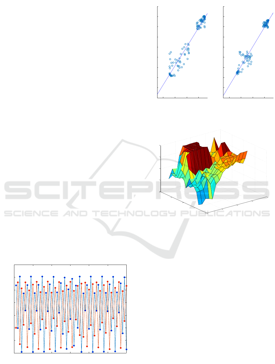
4.1.1 Near-periodicity and Bunching

We now return to the case in the upper right panel

in Figure 6. For

= 3.625

and

= 3.77

both logis-

tic maps—considered in isolation—are in the chaotic

phase, cf. Figure 2. But for

= 0.2

the dynamics of

y become nearly periodic as illustrated in Figure 7.

Nonlinear dynamic systems are known to display

intermittency (Ott, 2002), where periods of chaos are

interspersed with periods of nearly periodic behavior.

Intermittency, however, does not seem to be the cause

here, since the phenomenon persists no matter how

many points are discarded as transient before starting

300 310 320 330 340 350 360

0.3

0.4

0.5

0.6

0.7

0.8

0.9

, y

Figure 7: Plot of the time series of

(shown in blue) and

(shown in red) displaying nearly periodic behavior. Parame-

ter values: r

= 3.625, r

= 3.77, β

= 0, β

= 0.2.

0.2 0.4 0.6 0.8

0.1

0.2

0.3

0.4

0.5

0.6

0.7

0.8

0.9

ˆx|M

x,ˆx

= 0.96

0.2 0.4 0.6 0.8

0.1

0.2

0.3

0.4

0.5

0.6

0.7

0.8

0.9

ˆy|M

y,ˆy

= 0.97

Figure 8: Cross-mapped estimates vs. observed values of

and

. Parameter values:

= 3.625

= 3.77

= 0

= 0.2.

0.2

0.4

0.6

0.8

3.5

3.6

3.7

3.8

3.9

−1

−0.5

0.5

ρ(y)

Figure 9: Surface plot of

y ˆy

for

L = 400

as a function of

and

. Note that

is also varied, since

+ r

= 7.3984

= 0 throughout.

to sample. Instead, it seems, that

becomes partially

synchronized with

because the range of

-values lies

within several relatively narrow intervals. An example

of cross-mapped estimates for

and

are shown in

ﬁgure 8.

Near-periodicity results in

y ˆy

becoming higher

than

x ˆx

at low

, and ‘bunching’ of the points leads to

‘fast non-convergence’, i.e., high correlations, that are

not reminiscent of the convergence behavior expected

in CCM, evidenced by the fact that the ﬁts to

ρ(L)

Eq. 5 fail.

To see whether this is an isolated point in parameter

space, resulting in pathological behavior, we calculate

cross-mapped estimates

ˆy|M

for a range of param-

eter values

and

. For each value we discard

the ﬁrst 1000 points in the time series and sample

the next 400 points after that to construct the shadow

manifolds. The result is shown in Figure 9.

There is a clear plateau in Figure 9 that corresponds

Inferring Causality from Noisy Time Series Data - A Test of Convergent Cross-Mapping

to the ‘bunching’ observed in Figure 7, indicating that

the issue is not conﬁned to a few isolated parameter

combinations. Whether similar issues affect the use of

CCM for other models or when applied to empirical

data is a topic for future research.

4.2 Effects of Noise

Since all empirical data contain a certain level of noise

it is important to study what effect noise, as included

in Eq. 2, has on CCM results. We consider the simple

case of unidirectional coupling from

, i.e.,

= 0

In this case the noise term

x,t

propagates directly to

the variable

, and therefore does not affect the cross-

mapped estimates of

based on

(a fact that has

been veriﬁed by numerical simulations). On the other

hand, noise in

is not coupled back into

and could

potentially be detrimental to the reconstruction. Hence,

we will make the simplifying assumption of setting

x,t

= 0

. This leaves

,β

and the noise level

free parameters of the model in Eq. 2. We ﬁx

= 3.8

and

= 3.5

, so that

is in the chaotic regime and the

dynamics of

is governed by a period-4 attractor for

= 0

, but as illustrated in Figure 2 the dynamics of

will become increasingly chaotic as

increases. We

present results for three different values of

ranging

from weak to strong coupling. At low noise levels

CCM gives the correct result for all three values of the

coupling strength, namely that x causes y.

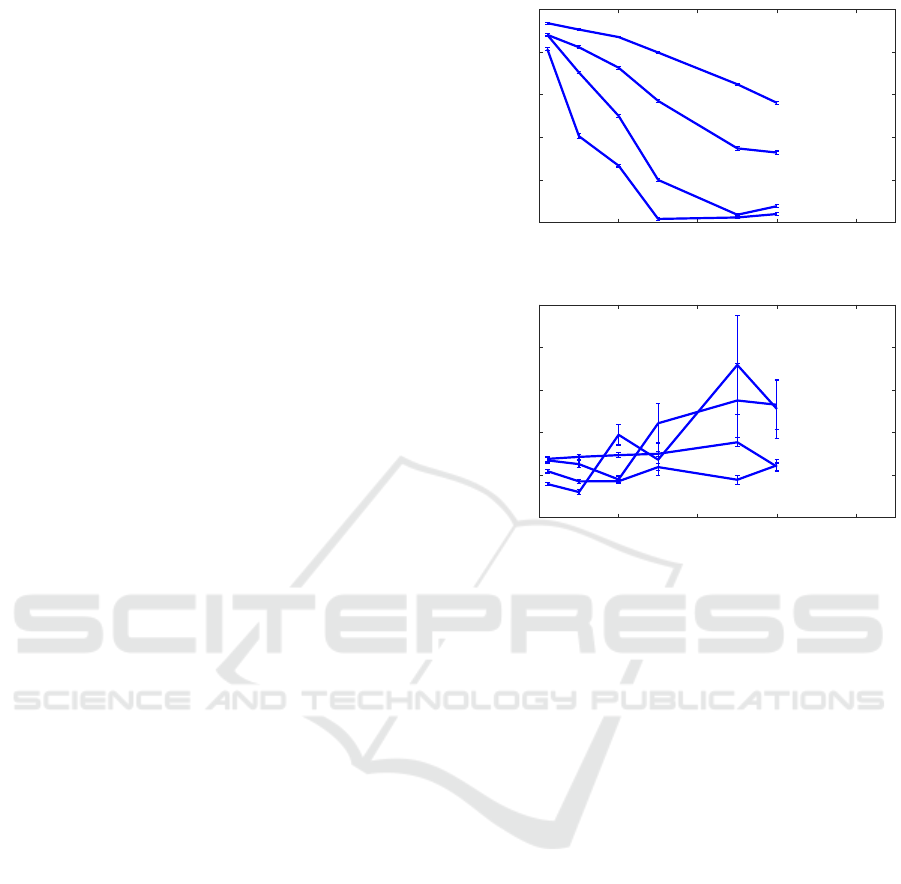
When the noise level

is increased the cross-

mapped estimates of

from

deteriorate, and as a

result

x ˆx

decreases. Figure 10 shows the ﬁtted values

x,∞

that

x ˆx

converges to as a function of the noise

level (top panel).

We see that

x,∞

decreases in a roughly linear fash-

ion as

is increased until the correlation becomes

very low

(0 . ρ

x,∞

. 0.2)

where the curve becomes

ﬂat. For systems corresponding to the ﬂat part of the

curves

x,∞

is very low and at about the same level as

y,∞

, so, effectively, the system is too noisy for CCM

to extract the direction of causality from the converged

value of ρ

x ˆx

The bottom panel shows that the rate of conver-

gence

from Eq. 5 is relatively unaffected by the

noise level, except when

x ˆx

≈ 0

, where CCM is not

applicable under any circumstances. But for combi-

nations of coupling strength and noise level that lie

on the linear decline of the curves in the top panel of

Figure 10 the ﬁtted rate of convergence

seems to

be a better indicator that

x ˆx

converges than

x,∞

; and

hence also a better predictor of causality.

0 0.01 0.02 0.03 0.04

0.2

0.4

0.6

0.8

x,∞

= 0.05

= 0.1

= 0.2

= 0.4

0 0.01 0.02 0.03 0.04

0.02

0.04

0.06

0.08

0.1

= 0.05

= 0.1

= 0.2

= 0.4

Figure 10: The effect of the noise level

on the converged

value

x,∞

x ˆx

(top panel) and on the rate of convergence

x ˆx

(bottom panel). In all cases

= 3.8

= 3.5

and

= 0

. The coupling

was varied as shown in the ﬁgure.

The error bars represent 95% conﬁdence intervals on the

ﬁtted values.

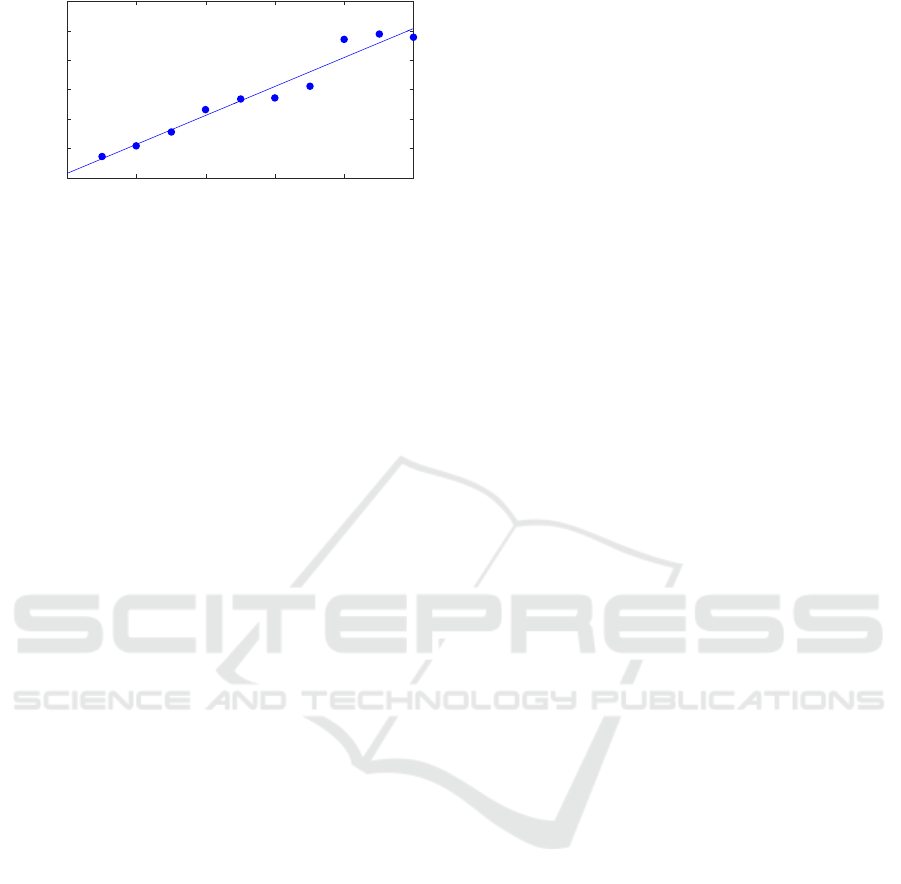
4.2.1 Estimating Coupling from Noise

As noted above, we observe from Figure 10 that

x,∞

decreases linearly as a function of noise. We further

note that the inverse of the slope depends linearly on

the strength of the coupling, as shown in Figure 11.

For the particular example studied here this has the

implication that we can determine the strength of the

coupling from

by controlled injection of noise

into the system. Whether this results generalizes to

other systems is a question for future research that has

practical implications for measuring the interaction

between different parts of complex dynamic systems.

5 DISCUSSION

Methods for reliable inference of causality between

two or more variables are of great interest to many

ﬁelds of research. Convergent Cross-Mapping (CCM)

shows great potential in this regard. However, based

on the systematic assessments presented in the previ-

ous sections, we conclude that the method can give

COMPLEXIS 2016 - 1st International Conference on Complex Information Systems

0 0.1 0.2 0.3 0.4 0.5

0.02

0.04

0.06

0.08

0.1

−1/q

Figure 11: The inverse negative slope

−1/q

of the linear

portion of the curves in the top panel of Figure 10 as a

function of the coupling.

erroneous results. It was noted already by Sugihara

et al. (2012) that CCM does not correctly predict the

direction of causality when the coupling is so strong

that it results in synchronization of variables, as we

have also seen above. Further, our study shows that

the method seems very sensitive to the particular dy-

namics of the model system, and CCM also fails to

correctly predict the direction of causality in cases

where the coupling is weak to moderate. Interestingly,

we have shown that both types of cases where CCM

fails is associated with a failure to ﬁt the observed val-

ues of cross-mapped correlations to the function

ρ(L)

in Eq. 5. It would therefore seem that the failure to

produce a good ﬁt to

ρ(L)

is an indicator that CCM is

not applicable to the data.

Another aspect of CCM performance concerns con-

ditions of noise. Generally, we observe that CCM is

fairly robust to random noise and makes reliable infer-

ences at varying degrees of coupling under conditions

of lower noise levels. However, for higher levels of

noise CCM correlations drop linearly as a function

of added noise. For systems subject to noise our re-

sults suggest that the rate of convergence is a more

robust indicator of cross-mapping convergence and

hence of causality. In applications where noise can

be controlled, injecting noise into the system at differ-

ent noise levels presents an opportunity to gauge the

strength of coupling between variables.

Together our results warrant caution in the applica-

tion of CCM to real-world data for purposes of causal

inference, and care must be taken to look in detail at

the convergence properties of the correlations between

observed data and cross-mapped estimates. Our re-

sults suggest that ﬁtting the correlation coefﬁcients

as a function of library length can give an indication

of the applicability of CCM. When applied under the

right circumstances, the method has the potential not

only to inform the researcher about the causal direc-

tion of dynamics between coupled variables, but by

controlled injection of noise, we can also infer the

coupling strength between the variables.

ACKNOWLEDGEMENTS

We would like to acknowledge the Interacting Minds

Centre, Aarhus University, for providing the ideal en-

vironment for the authors’ collaboration.

REFERENCES

Abarbanel, H. (1996). Analysis of Observed Chaotic Data.

Springer New York.

Boccaletti, S., Kurths, J., Osipov, G., Valladares, D. L., and

Zhou, C. S. (2002). The synchronization of chaotic

systems. Physics Reports, 366(1–2):1–101.

BozorgMagham, A. E., Motesharrei, S., Penny, S. G., and

Kalnay, E. (2015). Causality Analysis: Identifying

the Leading Element in a Coupled Dynamical System.

PLOS ONE, 10(6):e0131226.

Ferretti, A. and Rahman, N. K. (1988). A study of coupled

logistic map and its applications in chemical physics.

Chemical Physics, 119(2–3):275–288.

Fraser, A. M. and Swinney, H. L. (1986). Independent coor-

dinates for strange attractors from mutual information.

Physical Review A, 33(2):1134–1140.

Granger, C. W. J. (1969). Investigating Causal Relations

by Econometric Models and Cross-spectral Methods.

Econometrica, 37(3):424–438.

Jespersen, S. N. (2013). Personal communication.

Kantz, H. and Schreiber, T. (1997). Nonlinear Time Series

Analysis. Cambridge University Press, New York,USA.

Lakoff, G. (2010). Why it Matters How we Frame the Envi-

ronment. Environmental Communication,4(1):70–81

Lloyd, A. L. (1995). The coupled logistic map: a sim-

ple model for the effects of spatial heterogeneity on

population dynamics. Journal of Theoretical Biology,

173(3):217–230.

Ma, H., Aihara, K., and Chen, L. (2014). Detecting Causality

from Nonlinear Dynamics with Short-term Time Series.

Scientiﬁc Reports, 4:7464.

Marwan, N., Carmen Romano, M., Thiel, M., and Kurths, J.

(2007). Recurrence plots for the analysis of complex

systems. Physics Reports, 438(5–6):237–329.

May, R. M. (1976). Simple mathematical models with very

complicated dynamics. Nature, 261(5560):459–467.

McBride, J. C., Zhao, X., Munro, N. B., Jicha, G. A.,

Schmitt, F. A., Kryscio, R. J., Smith, C. D., and Jiang,

Y. (2015). Sugihara causality analysis of scalp EEG for

detection of early Alzheimer’s disease. NeuroImage:

Clinical, 7:258–265.

McCracken, J. M. and Weigel, R. S. (2014). Conver-

gent cross-mapping and pairwise asymmetric inference.

Physical Review E, 90(6):062903.

Mønster, D. (2013). XMAP. https://github.com/danm0nster

/xmap.

Moran, P. (1953). The statistical analysis of the Canadian

Lynx cycle. Australian Journal of Zoology, 1(3):291–

298.

Inferring Causality from Noisy Time Series Data - A Test of Convergent Cross-Mapping

Ott, E. (2002). Chaos in Dynamical Systems. Cambridge

University Press, Cambridge, U.K. ; New York, 2 edi-

tion edition.

Pearl, J. (2009). Causal inference in statistics: An overview.

Statistics Surveys, 3:96–146.

Pikovsky, A., Rosenblum, M., and Kurths, J. (2003). Syn-

chronization: A Universal Concept in Nonlinear Sci-

ences. Cambridge University Press.

Schreiber, T. (2000). Measuring Information Transfer. Phys-

ical Review Letters, 85(2):461–464.

Sugihara, G., May, R., Ye, H., Hsieh, C.-h., Deyle, E., Foga-

rty, M., and Munch, S. (2012). Detecting Causality in

Complex Ecosystems. Science, 338(6106):496–500.

Sugihara, G. and May, R. M. (1990). Nonlinear forecasting

as a way of distinguishing chaos from measurement

error in time series. Nature, 344(6268):734–741.

Takens, F. (1981). Detecting strange attractors in turbulence.

Lecture Notes in Mathematics, 898:366–381.

Webber, C. L. and Zbilut, J. P. (1994). Dynamical assess-

ment of physiological systems and states using recur-

rence plot strategies. Journal of Applied Physiology,

76(2):965–973.

COMPLEXIS 2016 - 1st International Conference on Complex Information Systems