Finding Most Frequent Path based on Stratiﬁed Urban Roads

Enquan Ge, Jian Xu, Ming Xu, Ning Zheng, Weige Wang and Xinyu Zhang

School of Computer Science and Technology, Hangzhou Dianzi University, Hangzhou, China

Keywords:

Path Query, Upgrade Points, Road Levels, Trajectory Data, Stratiﬁed Urban Roads.

Abstract:

The path query based on big trajectory data has become a promising research direction due to the rapid de-

velopment of the Internet. Previous studies mainly focus on searching paths in full road network and ignore

the importance of stratiﬁed urban roads. It is observed that higher-level roads gather more trajectory points

which means most drivers prefer the high-level road. In this paper, we study a new path query to ﬁnd the

most frequent path (MFP) based on road levels in large-scale historical trajectory data. We refer to this query

as most frequent path based on road levels (RLMFP). Intuitively, selecting roads which are in line with local

custom and choosing high-level roads such as high-way are people’s two common sense notions. Our query

not only satisﬁes aforementioned sense, but also has two advantages in algorithm implementation. First, the

road hierarchy can speed up the path query. Next, the trajectory data can ﬁnd more reasonable upgrade points

(e.g., path query based on road levels need to ﬁnd the intersection between low-level roads and high-level

roads). Experiments show the effectiveness and the efﬁciency of our method.

1 INTRODUCTION

With the increasing amount of available information

in Internet, our society has entered a new period of

information technology. In our daily life, the number

of Global Positioning System (GPS) and devices with

wireless interactive system such as mobile phones,

navigation systems and emergency communications

are increasing quickly. These Location-Based Ser-

vices (LBS) have become increasingly popular. The

demand for such services is also rising, especially

the requirements of recommended route. Speciﬁcally,

given a source S, a destination D and a map, a recom-

mended route system is able to ﬁnd a path from S to

D in a map.

In recent years, a large number of mobile devices

and navigation devices also surge to generate trajec-

tory data, so more and more people begin to focus on

the study of path query with historical trajectory. His-

torical trajectory data can represent the users’driving

habits which are very signiﬁcant for the path query.

For example, when tourists arrive in an unfamiliar

place and get lost, what they want to do is to ask

a local person rather than use navigation equipment.

Though this path is not the fastest one or the shortest

one, it is the most suitable in a combination of time,

length and road conditions (Su et al., 2014). Thus if a

path query system returns a route based on historical

trajectory data, it also imply the local drivers’ path se-

lection habits. This is the ﬁrst requirement that a nav-

igation system must meet. Researchers (Luo et al.,

2013)(Chen et al., 2011) have provided methods to

solve it. Another requirement is that users wish to

pass through fewer junctions and drive on better roads

(e.g., freeway or highway). Figure 1 is a partial road

network of Beijing. The set of purple points are the

real trajectory data of taxi drivers, we get the trajec-

tories from (Yuan et al., 2011). This is a sample of

T-Drive trajectory data that contains one-week trajec-

tories of 10,357 taxis. Some of them are presented

on the map of Beijing in Figure 1. We can see that

more drivers prefer higher level roads. Note that there

are less intersections and trafﬁc lights on higher level

roads. Besides, when drivers use a navigation equip-

ment which provides a path with many intersections

and lanes, it is easy for them to take a wrong way or

miss intersections they need to turn. Previous meth-

ods generally search a path on the whole map. There-

fore, they may be insensitive to road levels and could

not meet the second requirement. Note if an algorithm

is searching based on the full map and the map con-

tains a huge number of intersections and roads, the

conventional methods would spend a large amount of

search time.

We study a novel method named most frequent

path based on road levels (RLMFP). Most frequent

paths (MFP) (Luo et al., 2013) use trajectories to rec-

ommend path. Different from other algorithms, the

Ge, E., Xu, J., Xu, M., Zheng, N., Wang, W. and Zhang, X.

Finding Most Frequent Path based on Stratiﬁed Urban Roads.

In Proceedings of the 2nd International Conference on Geographical Information Systems Theor y, Applications and Management (GISTAM 2016), pages 51-60

ISBN: 978-989-758-188-5

Figure 1: Partial map of Beijing.

weight of an edge in MFP is deﬁned as counting

the number of the trajectories passing through this

edge. This weight of a map is named as edge fre-

quently. And the weight of a path is a sequence ob-

tained by sorting all the edge weights of P in non-

decreasing order. For example, there are ﬁve edges

in P and their weights are (5,3,6,4,7). So the weight

of this path is (3,4,5,6,7). Similarly, another path P

is (2,6,7,8,9,11). P is better than P

in MFP because

3(the ﬁrst weight of P) is bigger than 2(the ﬁrst weight

of P). It can well meet the ﬁrst requirement of users

for the path ﬁnding. This method of judging a bet-

ter path is used by RLMFP. Here road level means

the level of a road in a city. Many cities have their

own plan and make roads into several levels accord-

ing to their states, roles and trafﬁc function. For in-

stance, roads of China and Unites States are classiﬁed

into 4 levels, and those of European Union are clas-

siﬁed even into 13 levels. The roads of each level

have different functions and properties. For example,

the function of highways is to connect multiple large

regions and the properties of highways deﬁne the de-

sign speed (60-80km / h), the number of one-way road

(≥4) and the width of total road (40-70m). In this pa-

per we use the nature road levels to speed up the path

searching and select high-level road segment to meet

the second demand.

In brief, our algorithm ﬁrst associate level proper-

ties to the vertexes and edges of road networks , then

judges the area where the start point (end point) lies

in and then determines the highest level of road net-

work and the upgrade points (i.e., the points connect-

ing edges in different levels). After that it uses MFP

to ﬁnd all sub-paths in the area. At last, we combine

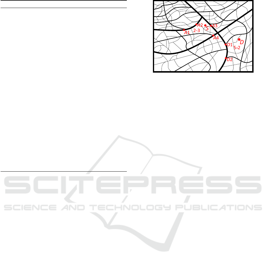
all sub-paths and chooses the best one. As shown in

Figure 3, A1,A2,A3 and A4 are the upgrade points of

S in area(2 − 3). Similarly to S, D1 and D2 are the

upgrade points of D. The rough(thin) edges represent

high(low) level roads. Firstly, we get the S.area and

D.area. Here is area(2 − 3) and area(5 − 2). Then

an index named FG(section 6) is used to ﬁnd a set of

best upgrade points from area(2 − 3) to area(5 − 2).

Assuming A3,A4 and D1 is selected. Then we use

MFP to compute the paths from A to A3,A4 , D to D1

in low level road networks and A3,A4 to D1 in high

level road. Then we combine these sub-paths. There

are two paths which are P1(A → A3 → D1 → D) and

P2(A → A4 → D1 → D). And ﬁnally, we select the

better paths with Deﬁnition 2.11. The details of algo-

rithm is given in following paragraphs.

So MFP algorithm considering road levels is fea-

sible, effective and evidence-based. But existing hier-

archical algorithm often layers for the convenience of

calculation ignoring the delamination characteristics

owned by the road itself. In this paper, aside from the

function of building a new road network, the trajec-

tory data is also used to determine the upgrade points.

We also construct an index of all upgrade points. This

can not only help correct direction, but also speed up

the algorithm.

Above all, our method is justiﬁed in reality and

validated in algorithm. The contributions of this paper

are the following.

• We propose a novel path query named most fre-

quent path based on road levels (RLMFP).

• We present a hierarchical algorithm to solve

RLMFP problem.

• We present an algorithm to build the index struc-

ture of upgrade points (FG).

• We develop a new hierarchical algorithm to solve

RLMFP problem using the index structure of up-

grade points (RLMFPT).

The rest of this paper is organized as follows.

First, we brieﬂy introduce a four-step framework to

solve the RLMFP problem in the context of very large

trajectory data sets (Section 2). Second, we provide

an algorithm to build a weighted road networks (Sec-

tion 3). Third, we explain area division (Section 4).

Fourth, we present a hierarchical algorithm to solve

RLMFP (Section 5). Fifth, we propose a method to

build the index structure of upgrade points. Sixth, we

develop a new hierarchical algorithm to solve PLMFP

utilizing the index structure of upgrade points (Sec-

tion 6). Then we present the experimental results

(Section 7). Next, we review the related work. We

conclude the paper in (Section 8).

GISTAM 2016 - 2nd International Conference on Geographical Information Systems Theory, Applications and Management

Table 1: Summary of Notations.

Notation Description

G,P,Y road network, path, trajectory

V ,E set of vertex(points), set of edge(roads)

G(i),V (i),E(i) i–level of G,V,E

X path or trajectory

X.s/X.d starting/ending vertex of X

X[i] the i–th element of X

T set of trajectory

F(u,v) frequency of edge (u,v)

F(P) frequency of path P

int(q) set of q–level upgrade vertices

NG new graph with trajectory data

FG an index for upgrade points set

S.area(q) the area for point S in q–level graph

P(area)/area(P) the area for point P

Area[i] the i–th area of graph

2 THE RLMFP PROBLEM

2.1 Problem Formulation

In previous section, two key requirements for path

query are provided from the users.

Property 2.1 (Local Drivers Path Selection). Select-

ing roads which are in line with local custom.

Property 2.2 (Better Roads). The roads with less in-

tersections and high-level road.

We have showed that the path from trajectory data

can meet Property 2.1 and the algorithm based on

road levels can satisfy Property 2.2. The deﬁnition of

RLMFP should satisfy the above 2 key requirements.

Here follows the formal deﬁnition. For clarity, the

main notations used in the rest of this paper are sum-

marized in Table 1.

Deﬁnition 2.1 (Road Network). A road network is a

directed graph G = (V,E) where V represents the set

of road intersections and E represents the set of road

segments.

Figure 1 presents a partial road network of Bei-

jing.

Deﬁnition 2.2 (Path). Given G, path P is a set of con-

sequent roads E

= {(x

),(x

),.. ., (x

k−1

)} and intersections V

= (x

,.. ., x

) from x

. P is a subgraph of G and the x

are all distinct.

P.s, P.e, and P[i] are used to denote the source ver-

tex x

, the ending vertex x

, and the i-th vertex x

respectively. In addition, P is often represented by

P.s → P.e or P(x

→ x

→ ·· · → x

) in short, where

P.s (or P.e) represent x

(or x

Deﬁnition 2.3 (Trajectory). Given G, a trajectory Y

is a sequence ((y

),(y

),.. ., (y

)) such that

there exists a path y

→ y

→ ··· → y

on G and t

a time stamp indicating the time when Y passes y

Similar to path, Y.s, Y.e, and Y [i] are used to de-

note the source vertex y

, the ending vertex y

, and

the i–th vertex y

, respectively. In addition, Y is often

represented by Y.s → Y.e in short, where Y.s(or Y.e)

represent x

(or x

) or Y (x

→ x

→ · ·· → x

). We

denote T as the set of Y .

Deﬁnition 2.4 (Edge Frequency). Given G, T , and

an edge (u,v) ∈ G, the edge frequency F(u,v) is the

number of the trajectories containing (u,v).

Deﬁnition 2.5 (Trajectory Network). A road network

is a directed graph G = (V,E) where V represents the

set of road intersections, E represents the set of road

segments. We use W to represent the set of the weight

of each edge. In this paper, W is a set of the edge

frequency.

Deﬁnition 2.6 (Edge Level). Given a road network

G = (V,E), the level of an edge e is denoted as

e.level(i) according to the existing road network,

where i is the level of the road.

As shown in Figure 1, the yellow edges represent

the highest level edges and each level of them is 1

written as e.level(1).

Deﬁnition 2.7 (Vertex Level). The level of a vertex v

denoted v.level, is deﬁned as the highest level of all

edges to v. Vertex v is also written as v.level(i) when

the level of a vertex i is known.

As shown in Figure 1, the level of yellow edges is

e.level(1) and the level of buff edges is e.level(2). If

one vertex v is the intersection of the yellow edge and

the buff edge, the level of v takes the highest of edges

and here is v.level(1).

Deﬁnition 2.8 (Upgrade Vertex). A vertex v is an up-

grade vertex when the edges it connects are not in the

same level. The set of upgrade vertices in same level

is denoted as int(q) where q is the level.

As shown in Figure 3, A1 connected a 3-level edge

and a 2-level edge, so A1 is an upgrade vertex. If we

want to ﬁnd the path from S to D, then the upgrade

vertices A1,A2,A3,A4 belong to S.int(1).

Deﬁnition 2.9 (Layered Graph). Layered graph

G(i) = (V (i), E(i)) is a subgraph of G, to ∀e(or v) ∈

E(i)(or V (i)), e.level(or v.level) ≤ i.

As shown in Figure 2, G(2)is a road network G,

this is because the lowest level of G(2) is 2,so G(2)

contains all vertices and edges. Thus G(2) is G and

G(1), G(2) represents the graph of level 1 and level 2.

Deﬁnition 2.10 (Area). Given a graph G(i) =

(V (i),E(i)) ,dividing the G(i + 1) into several sub-

graph through E(i). Each area Area( j) is one

Finding Most Frequent Path based on Stratiﬁed Urban Roads

area of G(i + 1) where j ∈ (1,2, .. ., k). ∀e ∈

Area( j),e.level ≥ i +1.

As shown in Figure 2, G(1) using its edges to cut

G(2) into ﬁve areas. For any area, the level of its

edges is no smaller than 2.

Deﬁnition 2.11 (More-frequent-than Relation).

Given two path frequencies F(P) = ( f

,.. ., f

)

and F(P

) = ( f

,.. ., f

) w.r.t. the same trajectory

network, F(P) is more-frequent-than F(P), denoted

as F(P)  F(P), if one of the following statements

holds:

• F(P) is a preﬁx of F(P

);

• there exists a q ∈ 1,. .. ,min(m, n) such that 1) f

for all i ∈ 1,... ,q −1, if q > 1, and 2) f

> f

Particularly, F(P) is strictly-more-frequent-than

F(P

), denoted as F(P) > F(P

), if F(P)  F(P

) and

F(P) 6= F(P

Problem Statement: Given a graph G, trajectory

set T, source S and a destination D, the recommended

route system searches MFP based on road levels from

S to D.

2.2 Solution Overview

Most frequent path based on road levels has four

steps. It is shown in Algorithm 1. First, a large num-

ber of trajectory data should be matched to the road

network so as to construct a new road network where

the weight is edge frequency. Then we divide the

graph into different areas according to the natural road

levels. Next the trajectory data T and the stratiﬁed

graph G∗ are employed to build index FG (section 6).

Finally, we use the algorithm to search the RLMFP

and return the P.

The ﬁrst step of this algorithm is to build G∗,

which means make the trajectory data match the road

network. GPS data is a sequence of vertices made by

users, therefore the path depending on the trajectory

can reﬂect the choice of users. After building a new

graph, some methods (Luo et al., 2013)(Chen et al.,

2011) compute the path on whole road network di-

rectly. Though there are different ways in various al-

gorithms, each of them should scan the full road net-

work. Hence stratiﬁcation is introduced in this paper.

In step 2, G is divided into areas by road levels. For

example, the ﬁrst level road network G(1) is the high-

est. Then we utilize the edge of ﬁrst level to divide

G into areas where any edge of areas is lower than

1. The existing algorithm (Bast et al., 2006) must tra-

verse all upgrade vertices in the area. Here we em-

ploy the trajectory data to reduce the number of up-

graded vertices. After that, the areas, road levels and

upgrades vertices are determined according to detect

which area the start vertex and end vertex lie in. Fi-

nally, we can perform the RLMFP.

Algorithm 1: Five steps for the RLMFP query.

Require:

G: road network; T : trajectory data set; S: start point;

D: end point;

Ensure:

the RLMFP;

1: build a new road network G∗ w.r.t. T ;

2: divide G into areas w.r.t. road levels;

3: build an index FG w.r.t T and stratiﬁed graph in 2;

4: ﬁnd the RLMFP P from S to D;

5: return P;

3 CONSTRUCT WEIGHTED

ROAD NETWORK

In this section, we construct a weighted road network.

According to the Deﬁnition 2.5, the weight of an edge

is different in algorithms. The existing algorithms ad-

dress the weight with Euclidean distance (Bellman,

1958)(Dijkstra, 1959), network distance and speed.

In this paper the weight of one road segment is de-

termined by the times that users passed. It is obvious

that the path based on Euclidean distance means the

nearest path and the path based on speed means the

fastest path. However, in fact, some drivers may avoid

aforementioned paths due to their experience, for ex-

ample, when in a strange place, users prefer to believe

the local people rather than the navigation system (Su

et al., 2014).

Algorithm 2: Build weighted road network.

Require:

G: road network; T : trajectory data set;

Ensure:

G∗: new road network;

1: G∗ ← NG[V G][V G] matrix with all entries zeros;

2: for each Y in T do

3: match Y to G ;

4: get a path P corresponds Y in G ;

5: for each edge e in P do

6: search e in G∗;

7: NG.edge.weight + + ;

8: return NG;

The idea is to ﬁnd path depending on the history

trajectory data of the local residents. It is because the

local person drives in their familiar areas and trajec-

tory data record their driving habits. So the ﬁrst step is

to build a trajectory network. It is shown in Algorithm

GISTAM 2016 - 2nd International Conference on Geographical Information Systems Theory, Applications and Management

(a) G(1) = E(1) (b) G(1) = E(1) ∪ E(2)

Figure 2: Experiments of similarity, path points and query

time in three algorithms.

2. First of all, we set the weight of each edge 0(line

1). Then we scan each trajectory and match them to

G(line 2-3). Note that there will be a corresponding

path produced(line 4). Next each edge section of the

path are selected from NG and add 1 to the weight of

them. We repeat the last steps until all the trajectory

have been processed.

4 AREA DIVISION

Due to the idea based on stratiﬁcation, after the com-

pletion of constructing the new road network G∗, G∗

needs to be divided into areas. Though road levels

are used in previous researches, most of them do this

for the convenience of the calculation. In fact, roads

themselves have level property and they are produced

by the trafﬁc conditions, living areas, working areas,

etc. As shown in Figure 2, G(2) is a layered network.

Assuming that we divide road network into 2 lev-

els in Figure 2. According to the function of different

roads, the roads can be divided into ﬁrst-level roads

E(1)(e.g. highway, freeway)and second-level roads

E(2)(e.g. city roads). In this way, G∗ can be ex-

tracted into a two-level structure of network. Here

G(1) = E(1), G(2) = E(1) ∪ E(2). Those nodes lo-

cated in the same position of different-level graphs

and connect to edges in different levels become the

upgrade vertices, which ensure the conversion of the

roads between the different layers.

After the road stratiﬁcation, low-level road net-

works should be divided into some smaller areas ac-

cording to the level of the road network. In area-

partition process, the high-level graph is cut by its

edges and the areas from it are the ones of next graphs.

We adopt a ﬂood-ﬁlling algorithm (Gonzalez et al.,

2007) to divide the graphs. Firstly, get a random ver-

tex whose level is lower than the cutting edges. Then

apply Breadth-First-Traversal(BFS) to the point. Note

that if BFS encounters a vertex whose level equals to

the level of cutting edges, the vertex would not be-

come traversed one but would be an upgrade point of

this area. We refer to the set of upgrade points as

int(q) in their area, where q is the level of their area.

Process is repeated until there is no traversed point.

As shown in Figure 2, G(1) is dividing into several

areas which named 1,2 etc. according to its edges.

Here every area is the area of G(2) and its edge-level

is 2, its vertex-level is no lower than 2. Each area is

named as (high-level)-(low-level). For example, the

area which name is 1 − 2 represents that it belongs

to area − 1 of G(1) and area − 2 of G(2). This ap-

proach not only addresses the index direction and de-

cides which level of network should be selected, but

also helps build the structure of indexing in every two

areas.

5 STRATIFICATION

ALGORITHM

In this section, we explain a stratiﬁcation algorithm to

ﬁnd path from start point to end point. We refer to

this query as most frequent path based on road lev-

els (RLMFP). First, assuming that the start point S

and end point D are in different regions of the L

and

. If S and D are in different levels, we judge higher

level and upgrade the area of lower level to higher

level graph until they are in the same level. Then we

judge whether they are in same area. If not, we repeat

this work till they are in same level and area. In this

way, the highest level road network for S and D is de-

termined. Next the vertices and graphs are upgraded

according to the highest level road network for S and

D. The algorithm is shown in Algorithm 3.

Initially, the algorithm traverses S and D in map

to determine which areas they are in (line1-2). Then

it addresses the highest level network they are both

in and use level record the highest level (line 3-5). If

q == level which means their level is the highest, it

can directly calculate the best path through the MFP

in their common area and the path is saved by P.max

(line 6-8). Otherwise, every path is computed from

S (or D) to S.int(q)(or D.int(q))(line9-12) and level

minus 1. This is one process of upgrading points. Af-

ter the ﬁrst upgrading, if S and D are still in different

levels, continue to upgrade S and D in the same way.

Here we should compute every SP(the most frequent

path) from points in S.int(q + 1) to points in S.int(q)

till q equals level(line 13-17). At last, a set of paths

P can be gotten by connecting each sub-path from S

to D and P.max can be return through calculating the

ﬁnal weight of each path in P.

Assuming there are n vertices and m edges in a

network with 2 levels of roads. Each time the average

number of vertices of all the MFP to end is k. The area

including most points has i upgrade points, n

vertices

Finding Most Frequent Path based on Stratiﬁed Urban Roads

Algorithm 3: Stratiﬁcation algorithm.

Require:

G∗: road network(including q levels, road levels is

E(1), E(2), ..., E(q), etc.); S: start point; D: end point;

Ensure:

the path RLMFP;

1: search S and D in G∗;

2: get S.area(q)and D.area(q);

3: level,oldq ← q;

4: while S.area(level)! = D.area(level) do

5: level ← level −1;

6: if q == level then

7: get SP(S − D) in E(q);

8: P.max ← P(S, D);

9: else

10: get every SP(S,S.int(q)) in E(q);

11: get every SP(D,D.int(q)) in E(q);

12: q ← q − 1;

13: while q > level do

14: get every SP(S.int(q + 1),S.int(q))inE(q);

15: get every SP(D.int(q + 1),D.int(q))inE(q);

16: q ← q − 1;

17: get every SP(S.int(q),D.int(q)) in E(q);

18: for each SP(1) ∈ SP(S, S.int(oldq)),...,SP(k) ∈

SP(D,D.int(oldq)) do

19: P ←

∑

i=1

SP(i);

20: get P.max from all P;

21: return P.max;

and m

edges at most. Each time the average num-

ber of vertices of all the MFP to end is k

. In the ﬁrst

layer, there are n

points, m

edges. Each time the

average number of vertices of all the MFP to end is

. If we take MFP algorithm directly, the time com-

plexity is O(kmn). If we adopt a stratiﬁcation algo-

rithm in this section, the time complexity of travers-

ing each upgrade of S(or D) in S.area(2) is O(k

the time complexity of the second layer is 2O(k

In the second layer, we should compute S(or D) to

every upgrade points in S.area(1), so the time com-

plexity of the second layer is 2iO(k

). Similarly,

the time complexity of the ﬁrst layer is O(k

Finally, the road sections should be connected to a

whole path. Here the path combines with three road

sections and go through two upgrade points, so the

number of paths is i

and its time complexity of se-

lecting best paths is O(i

). Therefore the whole time

complexity is 2iO(k

) + O(

) + O(i

). Due

to property (k

 knm), it’s easy to con-

cluded that the time complexity of RLMFP is much

smaller than MFP. But there may be a situation that

is unsatisﬁed. If there are too many upgrade vertices

with respect to the points in area are too many, they

would affect the performance of the entire algorithm

and i will affect the time complexity of this work.

Figure 3: Upgrade points.

6 HIERARCHICAL

OPTIMIZATION ALGORITHM

As shown in last section, RLMFP is more efﬁcient

than the MFP, but the number of upgrade points will

affect the time complexity. Worse still, due to the

global optimum road hierarchical algorithm, most of

the upgrade points being traversed are inappropriate.

As shown in Figure 3, A1, A2, A3 and A4 are the up-

grades of S in area(2 − 3). In stratiﬁcation algorithm,

we need to scan all paths from S to upgrade vertices.

But it is obvious that, people would choose the A3 or

A4 rather than A1 or A2. But the RLMFP in section 5

may upgrade road network through A1 or A2 because

MFP has no sense of direction. So the stratiﬁcation

algorithm has considered all paths, but there may be a

deviation for the best one and the number of upgrade

points has an impact on the time complexity.

In order to solve the problem, this paper provides

a hierarchical optimization algorithm RLMFPT, the

last T means terminal. As we know, the weight of

edge is based on trajectory, so we can simplify the al-

gorithm by selecting upgrade points according to tra-

jectory data.

The algorithm ﬁrst establishes an index table

to each of the two regions by storing a series

of upgrade points of different levels. We re-

fer to this index as FG. The storage structure is

, p

.nub),(p

, p

.nub),.. ., (p

, p

.nub). Here p

means the id of vertex, p

.num means the number of

being selected between the two areas. As shown in

Figure 3, if there is a trajectory from S to D and its re-

spect path pass the upgrade point A3, we plus 1 to the

A3.num in the index of area(2 − 3) and area(5 − 2).

We repeat it until all the trajectory is handled. The

algorithm is shown in Algorithm 4.

Firstly we construct an index structure and mark

all memory locations empty (line 1). The algo-

rithm then traverses all tracks and identiﬁes the ar-

eas of starting point and destination point to deter-

mine where to store in the index (line 2-3). Next,

GISTAM 2016 - 2nd International Conference on Geographical Information Systems Theory, Applications and Management

Algorithm 4: Build area index structure.

Require:

G: road network; T : trajectory data set;

Ensure:

FG: Area index structure

1: set all FG(area(G∗)∗ area(G∗)) with null;

2: for each Y in T do

3: get Y.s(area) and Y.d(area);

4: match Y to G ;

5: get a path P corresponds Y in G ;

6: for each point p in P do

7: if point p ∈ int then

8: push p to FG(area(Y.s))(area(Y.d));

9: area(Y.s)(Y.d).p.nub + +;

10: return FG;

each trajectory is matched to the network for obtain-

ing the appropriate paths (line 4-5). Finally, the al-

gorithm traverses every vertex on the path and judges

whether it is the upgraded one. If it is true, this point

will be stored in the position corresponding to the in-

dex construction. Assuming that the number of tra-

jectory data is |Y |, the number of points in the path

which each track corresponds to is |P|. The com-

plexity of the algorithm is O(|Y P|), space complexity

|area(G∗)|

Algorithm 5: Optimal Stratiﬁcation algorithm.

Require:

G∗: road network(including q levels, road levels is

E(1), E(2), ..., E(q), etc.); S: start point; D: end point;

FG: Area index structure;

Ensure:

the path RLMFPT;

1: search S and D in G∗;

2: get S.area(q)and D.area(q);

3: get FG(area(S)(D));

4: level,oldq ← q;

5: while S.area(level)! = D.area(level) do

6: level ← level −1;

7: if q == level then

8: get SP(S − D) in E(q);

9: P.max ← P(S, D);

10: else

11: get all S.int and D.int from FG(area(S)(D))

12: get every SP(S,S.int(q)) in E(q);

13: get every SP(D,D.int(q)) in E(q);

14: q ← q − 1;

15: while q > level do

16: get every SP(S.int(q + 1),S.int(q))inE(q);

17: get every SP(D.int(q + 1),D.int(q))inE(q);

18: q ← q − 1;

19: get every SP(S.int(q),D.int(q)) in E(q);

20: for each SP(1) ∈ SP(S, S.int(oldq)),...,SP(k) ∈

SP(D,D.int(oldq)) do

21: P ←

∑

i=1

SP(i);

22: get P.max from all P;

23: return P.max;

Different from the RLMFP, for the same condi-

tion, the algorithm determines the areas of start point

and end point and then determines the set of upgrade

vertices in FG. If upgrade vertices is in top 5 after

sorting their number, they are the upgrade ones of this

area. For example, FG(2 −3)(5 −2) has 100 upgrade

points(A1 − A100). We sort the number of points,

including A1.num, A2.num,..., A100.num. Then the

vertices in top 5 are selected as the upgrade ones.

The Algorithm 5 is similar to Algorithm 3. The

difference is getting the index in FG (line 3) and us-

ing the int(q) in FG(area(S)(D)) replace the int(q) in

area(line 11). The remaining part of the idea is same

as Algorithm 3.

Assuming the same condition of Algorithm 3, the

number of upgrade points is i

. And we have proved

that i

is among 5 to 10. The time complexity is

2iO(k

)+ O(k

)+ O(i

). Since i

is smaller

than i, thus the complexity is smaller than that of Al-

gorithm 3. In addition, because i

is a deﬁned low

value, it will not affect the time complexity. For ex-

ample, suppose each steps ratio of upgrade points is

cut to 30%, O(i

) is only 9% of O(i

). So the im-

proved results to Algorithm 3 is obvious.

7 EXPERIMENT

In this section we conduct experiment to compare

RLMFP, RLMFPT wiht MFP. In order to show ad-

vantages of RLMFPT, we design four experiments

for these three algorithms. Similarity is designed to

prove that RLMFPT has the advantages of MFP and

RLMFP, which means it satisﬁes Property 2.1. There

are more high-level roads in RLMFPT as a result of

natural hierarchical policy. A comparison of path

points is also done to prove that RLMFPT satisﬁes

Property 2.2. In addition, we compare the query time

of three algorithms to show the high query speed of

RLFMPT. At last, feasibility of RLMFPT is displayed

through the memory size of different algorithms.

In order to ensure the correctness and fairness of

the experiments, the trajectories is under the same

conditions. So We obtain trajectory data using the

famous Network-based Generator of Moving Objects

by Tomas Brinkhoff(Brinkhoff, 2002), which is a well

known system of generating trajectory data. In addi-

tion, the maps are Oldenburg and San Joaquin. The

smaller map Oldenburg has 6105 nodes and 7035

edges. The bigger map is San Joaquin with 18496

nodes and 24123 edges. In each map, we divide roads

into 2 levels. All the experiments are conducted on a

PC with an Intel CPU of 3.20GHz and 4GB memory.

Finding Most Frequent Path based on Stratiﬁed Urban Roads

(a) Similarity(OLD). (b) Similarity(SAN). (c) Path points(OLD).

(d) Path points(SAN). (e) Query time(OLD). (f) Query time(SAN).

Figure 4: Experiments of similarity, path points and query time in three algorithms.

7.1 Similarity

To evaluate the similarity of three path queries (MFP,

RLMFP and RLMFPT), we compare the results of

them through counting different quantities of the

same starting point and destination point path queries.

Due to the different sizes of the two maps, we pro-

duce 70000 and 510000 trajectories by trafﬁc simula-

tor as the data set for each of them. Then we set the

weights and build index FG for each graph with above

data set. Next we apply 10 to 100 path queries from

the same start point to the same end point for every

algorithm.

We use the ratio of the number of same edges in

two paths and the total number of edges in path which

is being com-pared. As shown in Figure 4(a) and Fig-

ure 4(b), there are about 40% of similarity between

MFP, RLMFP and RLMFPT, which indicates that the

similarity is relatively high. The difference is because

both RLMFP and RLMFPT traverse a high level map

when they get upgrade points, do not adapt MFP all

time. Because of the same principles and the high

similarity, it is shown that both RLMFP and RLMFPT

have the advantage of MFP and can satisfy the ﬁrst

demand of users. In addition, comparing RLMFP

with RLMFPT, there is high similarity between them.

Thus, RLMFPT (RLMFP with FG) has the advan-

tages of RLMFP.

7.2 Path Points

In this experiment, to evaluate the less number of

path points of RLMFP and RLMFPT, we compare the

results of them through counting different quantities

of the same starting point and destination point path

queries. The conditions are set up the same as 7.1.

As shown in Figure 4(c) and 4(d), with the in-

creasing number of queries, the number of points in

algorithms (RLMFP and RLMFPT) remains stable

between 30 and 35 in Figure 4(c) or 60 and 80 in Fig-

ure 4(d). The points of MFP gradually reduce with

the growing queries, but they are 50% more than that

of RLMFP or RLMFPT in Figure 4(d). It shows that

RLMFP and RLMFPT select less path points than

MFP, which satisﬁes the second demand of users.

7.3 Query Time

Algorithm proposed in this paper enjoy faster query

speed. Therefore, in this experiment, we compare

the results of the query time of three algorithms

(MFP, RLMFP, RLMFPT) through counting different

quantities of the same starting point and destination

point path queries to evaluate the less query time of

RLMFPT. The conditions are set up the same as 7.1.

As shown in Figure 4(e), with the increasing num-

ber of queries, the query time of MFP remains stable

at 7000ms. To the end point that have large number

of upgrade points, query time has ups and downs, be-

cause too many upgrade points would lead to a lot

of stitching path and affect the query time. Thus the

number of upgrade is an uncertain factor. But the

query time in 4(e) is still better than MFP. Besides,

because of the small number of upgrade points (less

than 9), the factor of that in RLMFP will not affect

RLMFPT. Therefore, the query time of RLMFPT still

remains at a relatively low state.

In large map San Joaquin shown in Figure 4(f),

as the number of queries increased, the query time of

MFP is decreasing and that of RLMFP is increasing.

GISTAM 2016 - 2nd International Conference on Geographical Information Systems Theory, Applications and Management

Figure 5: Memory size.

After stabilized,the query time of RLMFP is higher

than that of MFP. The reason is that the scale of up-

grade points is constantly increasing with the bigger

map, which affects the query time directly. In addi-

tion, the query time of RLMFPT still remains at a

short level. This is because the number of upgrade

points does not affect RLMFPT. Thus in San Joaquin

map, RLMFPT reﬂects the stable and short advan-

tages and also shows the advantages of FG.

7.4 Memory Size

In this experiment, we compare the results of the

memory size of common graph, stratiﬁed-graph and

FG by counting two maps to evaluate the acceptable

small extra memory size of RLMFPT.

As shown in Figure 5, regardless of the size of

maps, the memory size of stratiﬁed-graph is twice as

common graph. Besides, the memory size of FG is

similar to stratiﬁed graph and also twice as common

graph. Therefore, the memory size of RLMFPT is

about four times as common graph. In reality, such

additional storage is acceptable either on the client or

the server.

8 RELATED WORK

The best path algorithms have been studied for many

years. The most classic work is the shortest path algo-

rithm in the graph theory. (Dijkstra, 1959)(Bellman,

1958) propose two shortest path algorithms. These

algorithms have been studied for more than 50 years.

On the basis of these algorithms, the later researchers

develop some improved methods. (Pohl, 1971) pro-

poses bidirectional Dijkstra’s algorithm to improve

the efﬁciency of the algorithm. New approaches (Hart

et al., 1968) for fastest path ﬁnding are proposed aim-

ing at using heuristic information to reduce the time

complexity. In addition, if the weight on each edge

represents travel time, shortest path ﬁnding becomes

fastest path ﬁnding. (Kanoulas et al., 2006) raises

an idea that speed is changing in different time pe-

riods. He estimates the optimal departure time and

the shortest time depending on the property of each

edge. (Ding et al., 2008) also makes a way to ﬁnd

the fastest path under large graph. Due to the chang-

ing information in some roads, it may lead to update

whole road network so as to cause a huge waste of

resources. (Shang et al., 2010) uses two tree of prun-

ing map to solve the problems of update roads, which

effectively improves the memory utilization. Con-

sidering that clients may make too many requests in

the same period of time and lead to network con-

gestion, (Leong et al., 2014) broadcasts packets of

speed-changing weight. Then the client only accepts

needed data packets and compute paths in local. Dif-

ferent from shortest/fastest path querying, we study

the problem of ﬁnding the most frequent path. Thus

their methods for determining the better path are dif-

ferent and shortest/fastest path are not suitable for this

problem.

Finding a path utilizing the hierarchical road net-

work is another related work. (Geisberger et al., 2008)

offers CH algorithm, which ﬁrst orders all points and

compute this order to simplify the network gradually.

After pretreatment, it queries a path following the or-

der. Similar to (Geisberger et al., 2008), there are

many other methods through pretreating data such as

(Bast et al., 2006). (Bast et al., 2006) divides the

graph into many areas. When a point comes out from

the area, it should pass the access points. He prepro-

cesses all shortest paths between every pair areas for

optimization. But such approach has a defect that pre-

treatment time is too long. So (Akiba et al., 2013)

presents a large map of the road network under the

pruning techniques, resulting in great reducing of the

processing time. (Jing et al., 1996) proposes a hier-

archical road network to simplify algorithm. Though

these algorithms are searching a path according the

hierarchical idea, they are not focus on ﬁnding a path

based on stratiﬁed urban roads.

Querying a path based on trajectory data is the

most closely related work to this paper. Some

approaches (Gonzalez et al., 2007)(Yuan et al.,

2011)(Yuan et al., 2010)for fastest path ﬁnding are

proposed aiming at using user-generated GPS trajec-

tories to estimate the distribution of travel time on a

given road network. (Chen et al., 2011) recommends

a route by mining route preferences of the past visi-

tors. Specially, this method constructs a graph only

through trajectory clustering. He deﬁnes the possi-

bility of next point from query point to destination

point as the weight of graph. However, the method

may contain infrequent sub-path. (Luo et al., 2013)

proposes TPMFP to improve MPR. She utilizes edge

frequency as weight of graph. In addition, edge fre-

quency is computed in time of period, so the path do

not contain infrequent sub-path. (Su et al., 2014) is

Finding Most Frequent Path based on Stratiﬁed Urban Roads

the ﬁrst one who put local drivers advices into query

system. These methods are based on trajectories, but

they will lead to a high responding time due to search-

ing a path on a whole road network. In addition, a

path based on trajectories which favors the high-level

roads are ignored by these methods. They are there-

fore not a good method to ﬁnd a way based on trajec-

tory data.

9 CONCLUSION

In this paper, we propose two algorithms RLMFP and

RLMFPT (RLMFP with FG) to solve the problem

of path query. We observe two common sense no-

tions, which are selecting roads in line with local cus-

toms and choosing high-level roads such as highway.

Moreover, we study a four-step framework to solve

the problem. The ﬁrst step is to set the weight to the

common graph with trajectory graph. The second step

is to divide graph into several areas. The third step is

to build an index named FG to speed up the query and

ﬁnd more reasonable upgrade points. The last step is

to use RLMFPT to compute the paths. The experi-

ment results demonstrate the efﬁciency, the effective-

ness and the stability of our index FG and algorithm

RLMFPT. The memory size of RLMFPT is also ac-

ceptable for customers or providers. In the future, we

will extend our solution on real networks and recom-

mand custum made route via allowing drivers to select

preferable upgrade points.

ACKNOWLEDGEMENTS

This work is supported by the National Natural Sci-

ence Foundation of China (No. 61572165) and

the State Key Program of Zhejiang Province Nat-

ural Science Foundation of China under Grant No.

LZ15F020003.

REFERENCES

Akiba, T., Iwata, Y., and Yoshida, Y. (2013). Fast exact

shortest-path distance queries on large networks by

pruned landmark labeling. In Proceedings of the 2013

ACM SIGMOD International Conference on Manage-

ment of Data, pages 349–360.

Bast, H., Funke, S., Matijevic, D., Demetrescu, C., Gold-

berg, A., and Johnson, D. (2006). Transit: Ultrafast

shortest-path queries with linear-time preprocessing.

9th DIMACS Implementation Challenge — Shortest

Path / Demetrescu, Camil ; Goldberg, Andrew ; John-

son, David, (2006):175–192.

Bellman, R. (1958). On a routing problem. Quarterly Appl

Math, 16:87–90.

Brinkhoff, T. (2002). A framework for generating network-

based moving objects. Geoinformatica, 6(2):153–180.

Chen, Z., Shen, H.T., and Zhou,X.(2011). Discovering pop-

ular routes from trajectories. Icde,6791(9):900–911

Dijkstra, E.W.(1959), A note on two problems in connexion

with graphs. Numerische Mathematik,1(1):269–271

Ding, B., Yu, J. X., and Qin, L. (2008). Finding time-

dependent shortest paths over large graphs. Proc Edbt,

pages 205–216.

Geisberger, R., Sanders, P., Schultes, D., and Delling, D.

(2008). Contraction Hierarchies: Faster and Sim-

pler Hierarchical Routing in Road Networks. Springer

Berlin Heidelberg.

Gonzalez, H., Han, J., Li, X., Myslinska, M., and Sondag,

J. P. (2007). Adaptive fastest path computation on a

road network: A trafﬁc mining approach. In In Proc.

2007 Int. Conf. on Very Large Data Bases (VLDB07,

pages 794–805.

Hart, P. E., Nilsson, N. J., and Raphael, B. (1968). A formal

basis for the heuristic determination of minimum cost

paths. Systems Science & Cybernetics IEEE Transac-

tions on, 4(2):100–107.

Jing, N., Huang, Y. W., and Rundensteiner, E. A. (1996).

Hierarchical optimization of optimal path ﬁnding for

transportation applications. In In Proc of Acm Con-

ference on Information & Knowledge Management,

pages 261–268.

Kanoulas, E., Du, Y., Xia, T., and Zhang, D. (2006). Finding

fastest paths on a road network with speed patterns.

In In Proc. Int. Conf. on Data Engineering (ICDE06,

pages 10–10.

Leong, H. U., Zhao, H. J., Man, L. Y., Li, Y., and Gong,

Z. (2014). Towards online shortest path computation.

IEEE Transactions on Knowledge & Data Engineer-

ing, 26(4):1012–1025.

Luo, W., Tan, H., Chen, L., and Ni, L. M. (2013). Finding

time period-based most frequent path in big trajectory

data. In Proceedings of the 2013 ACM SIGMOD Inter-

national Conference on Management of Data, pages

713–724.

Pohl, I. (1971). Bi-directional search. Machine Intelli-

genceC, 6:1359–1364.

Shang, S., Deng, K., and Zheng, K. (2010). Efﬁcient best

path monitoring in road networks for instant local traf-

ﬁc information. In Conferences in Research and Prac-

tice in Information Technology Series, pages 47–56.

Su, H., Zheng, K., Huang, J., Jeung, H., Chen, L., and

Zhou, X. (2014). Crowdplanner: A crowd-based route

recommendation system. In 2014 IEEE 30th Inter-

national Conference on Data Engineering (ICDE),

pages 1144–1155.

Yuan, J., Zheng, Y., Xie, X., and Sun, G. (2011). Driv-

ing with knowledge from the physical world. Kdd,

pages316–324.

Yuan, J., Zheng, Y., Zhang, C., Xie, W., Xie, X., Sun,

G., and Huang, Y. (2010) T-drive: driving directions

based on taxi trajectories. In Proceedings of the 18th

SIGSPATIAL International conf. on advances in geo-

graphic information systems, pages 99–108 ACM.

GISTAM 2016 - 2nd International Conference on Geographical Information Systems Theory, Applications and Management