
Continuous Improvement of Proactive Event-driven Decision Making
through Sensor-Enabled Feedback (SEF)
Alexandros Bousdekis
1
, Nikos Papageorgiou
1
, Babis Magoutas
1
, Dimitris Apostolou
2
and Gregoris Mentzas
1
1
Information Management Unit, National Technical University of Athens, Athens, Greece
2
Department of Informatics, University of Piraeus, Piraeus, Greece
Keywords: Kalman Filter, Curve Fitting, Decision Support, Machine Learning, Manufacturing, Feedback.
Abstract: The incorporation of feedback in the proactive event-driven decision making can improve the
recommendations generated and be used to inform users online about the impact of the recommended action
following its implementation. We propose an approach for learning cost functions from Sensor-Enabled
Feedback (SEF) for the continuous improvement of proactive event-driven decision making. We suggest
using Kalman Filter, dynamic Curve Fitting and Extrapolation to update online (i.e. during action
implementation) cost functions of actions, with the aim to improve the parameters taken into account for
generating recommendations and thus, the recommendations themselves. We implemented our approach in
a real proactive manufacturing scenario and we conducted extensive experiments in order to validate its
effectiveness.
1 INTRODUCTION
Proactive, event-driven decision making is an
approach for deciding ahead of time about the
optimal action and the optimal time for its
implementation (Engel et al., 2012). Proactivity is
leveraged with novel information technologies that
enable decision making before a predicted critical
event occurs (Bousdekis et al., 2015). A proactive
event-driven Decision Support System (DSS) should
integrate different sensor data, provide real-time
processing of sensor data and combine historical and
domain knowledge with current data streams in
order to facilitate predictions and proactive
recommendations (Engel et al., 2012; Bousdekis et
al., 2015). The emergence of the Internet of Things
paves the way for enhancing the monitoring
capabilities of enterprises by means of extensive use
of sensors generating a multitude of data (Bousdekis
et al., 2015). The manufacturing domain can take
substantial advantage from proactive event-driven
decision making in order to turn maintenance
operations from “fail and fix” to “predict and
prevent” (Bousdekis et al., 2015). In addition, the
incorporation of feedback in the decision process
can, on the one hand, improve the recommendations
generated by the proactive event-driven DSS and, on
the other hand, be used to inform users online about
the impact of the recommended action following its
implementation. However, the noise existing in
manufacturing sensors makes proactive event-driven
decision making process vulnerable to inaccuracies.
Until now the embodiment of a feedback
functionality in proactive, event-driven decision
making has not been examined.
Our research objective is to examine how a
feedback loop can be implemented in a proactive
event-driven DSS so that data generated post action
implementation can be used to improve the decision
making process. Specifically, by focusing on
decision making processes that have a cost footprint
on the manufacturing process, we aim to investigate
how the cost functions of actions that are taken into
account for the provision of recommendations can
be updated and improved each time a recommended
action is implemented. Furthermore, we examine
what kind of data processing conducted by the
feedback loop is appropriate for informing online
users about the actual and the predicted cost of the
action during its implementation. Our approach is
followed by an application in a real industrial
environment and by extensive experiments for
validation.
The rest of the paper is organized as follows:
166
Bousdekis, A., Papageorgiou, N., Magoutas, B., Apostolou, D. and Mentzas, G.
Continuous Improvement of Proactive Event-driven Decision Making through Sensor-Enabled Feedback (SEF).
In Proceedings of the 18th International Conference on Enterprise Information Systems (ICEIS 2016) - Volume 2, pages 166-173
ISBN: 978-989-758-187-8
Copyright
c
2016 by SCITEPRESS – Science and Technology Publications, Lda. All rights reserved

Section 2 presents the related and background
works; Section 3 outlines our approach, while
Section 4 illustrates its application in a proactive
manufacturing scenario in the area of production of
automotive lighting equipment and presents
extensive experimental results in comparison to
Curve Fitting on noisy data, that prove the
effectiveness of our approach. Section 5 discusses
the results and concludes the paper.
2 RELATED AND BACKGROUND
WORKS
2.1 State-of-the-Art
There are several research works dealing with the
utilisation of feedback in Machine Learning
proposing algorithms based on Reinforcement
Learning (Lewis et al., 2012), iterative control
techniques (Lee and Lee, 2007), particle swarm
optimization (Tang et al., 2011) and incremental
learning (Chen et al., 2012). However, there is not a
methodology which enables the sensor noise
removal and the extraction of the function that these
sensor data follow in a way that can continuously
improve the recommendations provided by a
proactive event-driven system. Moreover, although
there are several applications in image processing
and robotics, learning from feedback has not been
used in order to update and improve costs of actions
that are expressed as a function of time. So, an
approach is needed for the continuous improvement
of a proactive event-driven system in terms of the
cost information that it handles, no matter which
decision method it uses.
For removing the noise from sensors and having
data closer to the real one, a Kalman Filter can be
used. Kalman Filters have been widely used for
removing noise in applications such as voltage
measurement, object tracking, navigation and
computer vision applications. Moreover, there are
some applications of Kalman Filters in prognosis of
manufacturing equipment (Sai Kiran et al., 2013).
However, a Kalman Filter is only able to provide the
corrected data based on the sensor measurements
and not to extract an estimation of the function that
these data follow. Curve fitting has been widely used
for extracting the linear, polynomial or exponential
function that a series of data follow and it can be
combined with extrapolation. However, when curve
fitting and extrapolation are applied to highly noisy
data, the level of confidence about the result is low,
since there is high uncertainty in both the actual
value of the measurement and the prediction that
extrapolation produces.
We argue that Kalman Filter, Curve Fitting and
extrapolation can be synergistically combined in
order to provide Sensor-Enabled Feedback (SEF) to
the decision making algorithms of a proactive event-
driven DSS about the actual cost functions that are
taken into account for the business performance
optimization and the provision of recommendations.
Although there are some research works proposing
such a combination, they address different problems
and in a different context (Sai Kiran et al., 2013),
while they assume the availability of historical data
or extensive domain knowledge (Yunfeng 2013).
2.2 Kalman Filter
Kalman Filter is an algorithm that uses a series of
measurements observed over time, containing
statistical noise and other inaccuracies in order to
provide estimations about the current values
(Kalman 1960). A Kalman filter is an optimal and
recursive estimator since it infers parameters of
interest from inaccurate observations as they arrive.
Moreover, it provides reliable results and is suitable
for online / real-time processing (Ertürk 2002). It is
suitable for linear systems, while, in cases of highly
non-linear systems, the Unscented Kalman Filter is
an accurate estimator (Kandepu et al., 2008).
Kalman Filter can be used for either uniform or non-
uniform sampling.
2.3 Curve Fitting and Extrapolation
Curve fitting is a numerical process that is used to
represent a set of experimentally measured (or
estimated) data points by some hypothetic analytical
functions (Vohnout 2003). Curve fitting can be
applied in several types of functions, e.g. linear (first
degree polynomial), polynomial, exponential. A
well-known curve fitting technique for linear
functions is the Linear Regression (Montgomery et
al., 2012). In the general form, for polynomial
functions, a widely used technique is Levenberg–
Marquardt algorithm (Lourakis 2005). For
exponential functions, a useful algorithm is Nelder-
Mead algorithm (Bűrmen 2006). Extrapolation
refers to the use of a fitted curve beyond the range of
the observed data and is subject to a degree of
uncertainty (Brezinski and Zaglia, 2013).
Extrapolation is implemented based on the curve
fitting results. Curve fitting and extrapolation can be
applied dynamically in a way that their output is
Continuous Improvement of Proactive Event-driven Decision Making through Sensor-Enabled Feedback (SEF)
167
updated in real-time as long as new data are gathered
from sensors.
3 OUR APPROACH
The overall approach for learning cost functions
from SEF for the continuous improvement of
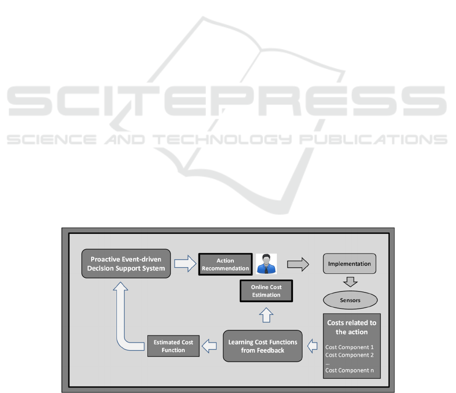
proactive event-driven DSS is shown in Figure 1.
The proactive event-driven DSS provides a
recommendation about the optimal action and the
optimal time for its implementation on the basis of a
prediction of a future undesired event, so that the
utility function is maximised (Engel et al., 2012).
For this reason, the decision making algorithms
embedded in the system take into account the
prediction but also domain knowledge, such as the
costs of actions as a function of time. The specific
algorithms used are not described here for brevity
but can be found in Bousdekis et al. (2015).
Cost functions are provided typically by domain
experts during the configuration of the system. In the
case of manufacturing, the total cost function is
typically an aggregation of different cost
components such as labour cost, cost due to
downtime, cost due to scrapped parts, cost due to
warranty claims, cost of spare parts, etc. (Amorim-
Melo et al., 2014). During the implementation of the
action, data regarding the cost functions can be
collected from different sensors (hardware,
software-e.g. ERP production plan- or human
sensors); their sampling may vary from the one cost
component to the other, while each cost component
may follow a different type of function (e.g. fixed,
linear, polynomial, exponential). The type of cost
functions may be affected either by the cost model
itself (e.g. labour cost is a linear function which
corresponds to a pay rate of X euros per hour) or by
a business process that causes a cost increase (e.g.
the number of defects per unit time affects the cost
function due to scrapped parts).
The process of learning cost functions from
feedback is shown in Figure 2. The figure provides a
more detailed explanation of the “Learning Cost
Functions from Feedback” block of Figure 1. For
each cost component, sensors generate noisy data
with a specific frequency either with uniform or with
non-uniform sampling. These noisy data include the
input of the Kalman Filter which removes the noise
and provides estimation about the current state (the
real current value of a cost component). In cases of
fixed and linear cost functions, the linear Kalman
Filter is used, while, for polynomial and exponential
cost functions, the Unscented Kalman Filter is used
(Kandepu et al., 2008). The Kalman Filter’s output
is provided as input to Curve Fitting, which is
applied during the implementation of the action and
is updated after every measurement. In case of fixed
and linear cost function, a linear regression
algorithm can be applied. In case of polynomial cost
function, a Levenberg–Marquardt algorithm can be
applied, while in case of exponential one, a Nelder-
Mead algorithm is suitable. The type of function has
been inserted into the system during its
configuration. Furthermore, at each measurement
time step, extrapolation is applied on the function
estimated by Curve Fitting in order to estimate the
future state of the system (i.e. future evolution of
cost function) until a pre-defined threshold. This
threshold can deal with the level of cost (e.g. the
action is going to stop in case of unpredictably high
costs, over a cost threshold) or the period of time (e.g.
the action is going to stop after a specific period of
time passes) or an average value of either cost or time.
Figure 1: Overall Approach.
ICEIS 2016 - 18th International Conference on Enterprise Information Systems
168

The process for learning cost functions is an
iterative process which takes place each time sensor
measurements exist. The user is informed online
about the estimated cost of action during its
implementation as shown in Figure 1. So, the user
becomes aware of the actual cost of the action and
its evolution until the end of the action. After the
implementation of the action, the updated cost
function of this action feeds into the proactive event-
driven DSS in order to be used in the next
recommendation in which this action is involved.
Figure 2: The process for learning cost functions from
feedback.
4 IMPLEMENTATION OF OUR
APPROACH
4.1 Application in a Real Industrial
Scenario
We validated our approach in a manufacturing
scenario in the area of production of automotive
lighting equipment. The production process includes
the production of the headlamps’ components. These
processes gather many data through embedded
quality assessment equipment using sensors and
measuring devices. A proactive event-driven DSS
embedding various decision methods would be able
to be developed based on a relevant architecture in
order to provide proactive recommendations
(Bousdekis et al., 2015). The proposed approach
could be coupled with such a proactive event-driven
DSS so that: (i) the user is informed online about the
estimated actual and future cost of action during its
implementation, and (ii) the updated cost function of
the specific action is used in the next recommendation
in which this action is involved. However, the cost
functions of actions that are taken into account for the
provision of recommendations are inserted in the
system only once, during the configuration stage
(Bousdekis et al., 2015) and the sensor measuring the
scrapped parts generates noisy data.
In the current scenario, there are two alternative
actions that can be recommended: the re-
configuration of the moulding machine during its
function (which results in higher scrap rate) or the
same action with downtime. The decision method of
the system calculates that the cost of production loss
due to downtime will be higher than the cost of
scrapped parts during moulding machine’s function.
So, the “re-configuration of the moulding machine
during its function” is the action that is
recommended along with the optimal time for its
implementation. This action may cause a
malfunction of the moulding machine which can
lead to an increase of scrapped parts during the
implementation. So, in this case, one cost component
exists: the cost due to the production of scrapped parts
when an action is implemented. The cost due to the
production of scrapped parts is represented by a linear
function. Each scrapped part has a cost of 100 € with
a constant rate at each time step equal to 1 scrapped
part per minute, as shown in Equation 1.
Cost Function = 100 * number of scrapped
parts * t
(1)
So, in this case, the noise exists in the number of
scrapped parts that the sensor measures during the
implementation of the action. Each time a part is
produced, the sensor sends a signal about whether it
is good or scrapped. When there is a signal of a
scrapped part, the cost of a unit part is added to the
cost till that time. The production rate of the
machine does not change, so there is a uniform
sampling since each time a part is produced, a
measurement is taken by a sensor. Based on domain
knowledge, the action will last approximately 2
hours. The function that has been given during the
configuration of the system is shown in Equation 2:
Cost = 100 * t (2)
Based on technical specifications and domain
knowledge, the sensor noise covariance for this
setup is equal to 6, therefore the cost noise
covariance will be:
Cost Noise Covariance = 6 * 100 € (3)
This has been calculated according to the formula:
Cost Noise Covariance = Sensor Noise
Covariance * unit cost
(4)
Continuous Improvement of Proactive Event-driven Decision Making through Sensor-Enabled Feedback (SEF)
169
The formulation of Kalman Filter is similar to a
position-constant velocity problem (Won et al.,
2010), but instead of position and velocity, there is
cost and rate of cost change. So, the equations of
Kalman Filter are modified accordingly. The
proposed approach was implemented in Python
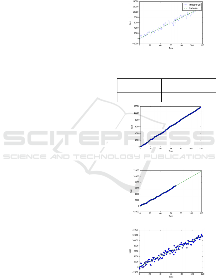
programming language. Figure 3 shows the
evolution of cost according to the noisy
measurements and according to the corrected
measurements after the implementation of Kalman
Filter. Since Kalman Filter cannot extract the
function, our approach applies dynamic curve fitting
in each iteration and in the final result. So, in this
example, linear regression is applied on the basis of
the points extracted from Kalman. The final result is
shown in Figure 4, where the output of the Kalman
Filter are data that approach a linear function and is
close to the line that linear regression creates.
The output of linear regression in the corrected
data is shown in Table 1. The equation is derived
from the results of Linear Regression about the slope
and the intercept (Montgomery et al., 2012). In this
example, R
2
is high and approaches 1, so the data
are fitted almost perfectly to the regression line. P-
value approaches 0, which means that the null
hypothesis can be rejected. Standard error is
0.225229389344, so the distance that the values fall
from the regression line is relatively low. The
sample size is equal to 120 as measurements are
taken every minute for 2 hours.
The final results, after the implementation of the
action, feeds into the proactive event-driven DSS
and updates the cost function of the specific action
which will be used in the next recommendation in
which this action is involved. At the same time, the
user is informed online about the estimated cost of
action during its implementation. This means that he
/ she is able to see the actual cost and its evolution
until now (through dynamic curve fitting) as well as
the estimated cost until a time threshold which in
this example is 2 hours (through extrapolation).
Figure 5 shows the dynamic curve fitting and
extrapolation technique at a specific time step of the
action implementation.
Since the objective is to extract the actual cost
function, we compare the results of our approach
with applying linear regression directly on the basis
of noisy data. This result is shown in Figure 6. The
output of linear regression in the corrected data is
shown in Table 2. R
2
is lower than the one in our
approach, so the data are fitted worse to the regression
line. P-value also approaches 0, but is slightly higher
than the one in our approach. Standard error is
1.79130743211, so the distance that the values fall
from the regression line is higher. The linear
regression is applied in the same sample size.
Figure 3: Cost evolution during the implementation of the
action.
Table 1: Output of curve fitting (linear regression) in the
corrected data for the scenario.
Equation
98.55 * t + 37.64
R
2
0.999384074129
P value
2.80148856911e-191
Standard Error
0.225229389344
Sample size
120
Figure 4: Curve Fitting (Linear Regression) on the basis of
corrected data.
Figure 5: Dynamic Curve Fitting and Extrapolation
Figure 6: Curve Fitting (Linear Regression) on the basis of
noisy data.
ICEIS 2016 - 18th International Conference on Enterprise Information Systems
170
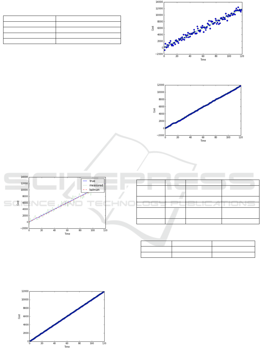
Table 2: Output of linear regression in the noisy data for
the scenario.
Equation
96.45 * t + 63.34
R
2
0.961777688176
P value
1.69862696613e-85
Standard Error
1.79130743211
Sample size
120
4.2 Experimental Results
4.2.1 Indicative Simulation Experiment
In order to validate the effectiveness of our
approach, we conducted simulations with various
noise levels and linear functions and we compared
the Mean Squared Error (MSE) and the Mean
Absolute Error (MAE) (Willmott, and Matsuura,
2005). The results show that our approach works
much better than applying linear regression on the
basis of noisy data. In other words, the resulting cost
function of our approach is closer to the true one
than the one of the linear regression applied to noisy
data. Figure 7 shows the results of one of the
simulation experiments. It shows the true function,
the measured noisy data and the data after the
implementation of Kalman Filter.
Figure 7: Result of a simulation experiment.
We applied Linear Regression to all the three
functions and the results for each one are shown in
Figure 8, in Figure 9 and in Figure 10. The output
results of Linear Regression are shown in Table 3.
Obviously, in the true function all the data fit
Figure 8: Curve Fitting (Linear Regression) on the basis of
the true data for the simulation example.
Figure 9: Curve Fitting (Linear Regression) on the basis of
the noisy data for the simulation example.
Figure 10: Curve Fitting (Linear Regression) on the basis
of corrected data for the simulation example.
Table 3: Output results of Linear Regression in the
simulation example.
True Measured Kalman
Equation
100 * t 98.65 * t +
78.76
98.66 * t - 22.79
R
2
1.0 0.973573107 0.999678
P value
0.0 5.92e-95 6.407e-208
Standard
Error
0.0 1.496 0.1629
Sample size
120 120 120
Table 4: Comparison of MSE and MAE.
Measured Kalman
MSE
433872.211071 12492.8947745
MAE
542.908521255 85.4088944024
perfectly to the regression line. The application of
Linear Regression on the basis of the data processed
by Kalman Filter gives better results. The plot data
are less scattered and more accurate due to the
application of Kalman Filter. This can also be
concluded by Table 4, which shows the values of
MSE and MAE of the two comparing approaches.
4.2.2 Overview of Experimental Results
In the simulation experiments, we applied Curve
Fitting on the basis of the measured noisy data and
on the basis of the corrected data (after the
implementation of Kalman Filter) for various Cost
Noise Covariances and Cost Functions. The results
Continuous Improvement of Proactive Event-driven Decision Making through Sensor-Enabled Feedback (SEF)
171
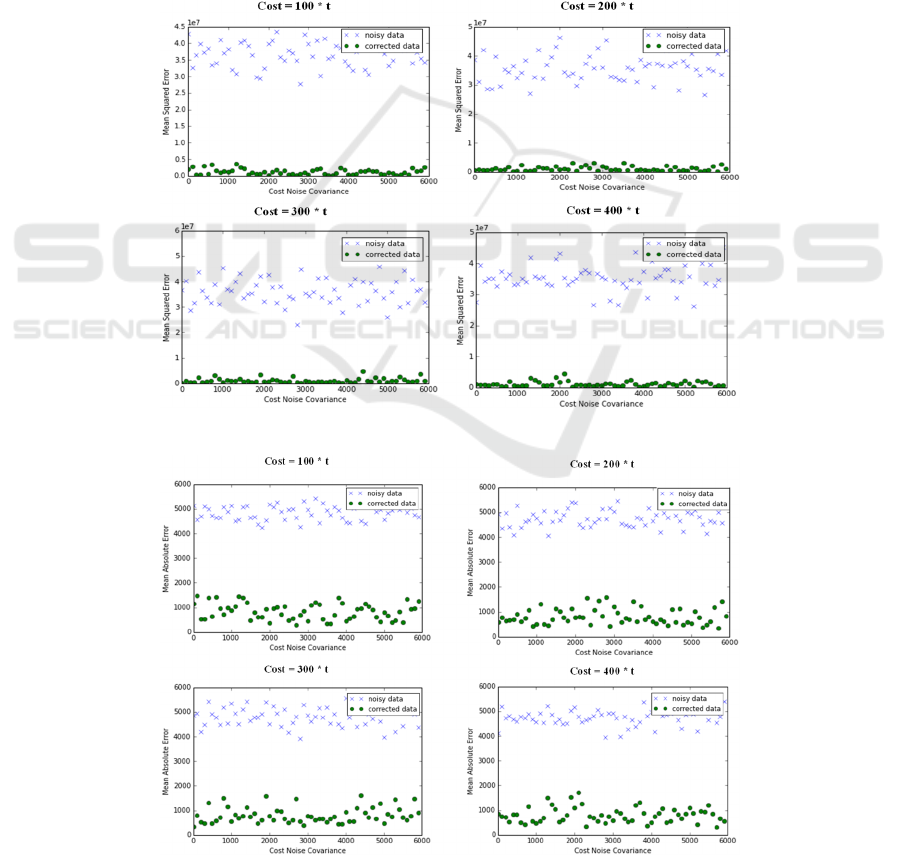
show that our approach provides more accurate
results. This was concluded by comparing the
resulting equations of the two approaches with the
true one. Thus, MSE and MAE were compared for
different Cost Functions and Cost Noise
Covariances, as shown in Figure 11 and in Figure 12
respectively. MSE and MAE of our approach is
always much lower for various Cost Noise
Covariances and for different Cost Functions.
5 CONCLUSIONS AND FUTURE
WORK
We propose an approach for learning cost functions
from SEF for the continuous improvement of
proactive event-driven decision making. We suggest
using Kalman Filter to update online cost functions
of actions, with the aim to improve the parameters
taken into account for generating recommendations
and thus, the recommendations themselves. More
specifically, our approach utilizes the capabilities of
Kalman Filter for removing noise from sensor data,
dynamic curve fitting on the basis of the corrected
data for extracting at each time step the cost function
and extrapolation on the basis of the corrected data
for predicting the evolution of cost until the end of
the implementation of the recommended action in an
accurate and reliable way. The SEF is received
during the recommended action implementation.
Figure 11: MSE for different Cost Functions and Cost Noise Covariances.
Figure 12: MAE for different Cost Functions and Cost Noise Covariances.
ICEIS 2016 - 18th International Conference on Enterprise Information Systems
172

The role of SEF is twofold: (i) The user is informed
online about the estimated cost of action during its
implementation, and (ii) The updated cost function
of the specific action is used in the next
recommendation in which this action is involved.
The proposed approach was tested in a real
industrial environment. In addition, simulation
experiments were conducted in order to prove its
effectiveness. Curve Fitting and extrapolation on
less noisy data (after the implementation of Kalman
Filter) gives more reliable results comparing to its
application to the sensor noisy measurements. In
other words, applying curve fitting in more accurate
and less noisy data can give a better insight about
the function that these data follow and can provide
more reliable predictions about the future values
through extrapolation. Regarding our future work,
we aim to add more cost models and validate our
approach for different functions for both uniform
and non-uniform sampling. Cost components may be
gathered from different sensors in a different
frequency, while some of them may conduct
uniform sampling and others non-uniform sampling.
We aim to examine the combination of all these
sensors and the aggregation of the total cost at each
time step.
ACKNOWLEDGEMENTS
This work is partly funded by the European
Commission project FP7 STREP ProaSense “The
Proactive Sensing Enterprise” (612329).
REFERENCES
Amorim-Melo, P., Shehab, E., Kirkwood, L., Baguley, P.
(2014). Cost Drivers of Integrated Maintenance in
High-value Systems. Procedia CIRP, 22, 152-156.
Bousdekis, A., Papageorgiou, N., Magoutas, B.,
Apostolou, D., Mentzas, G., 2015. A Real-Time
Architecture for Proactive Decision Making in
Manufacturing Enterprises. In On the Move to
Meaningful Internet Systems: OTM 2015 Workshops
(pp. 137-146). Springer International Publishing.
Brezinski, C., Zaglia, M. R., 2013. Extrapolation methods:
theory and practice. Elsevier.
Bűrmen, Á., Puhan, J., Tuma, T., 2006. Grid restrained
nelder-mead algorithm. Computational Optimization
and Applications, 34(3), 359-375.
Chen, X., Huang, J., Wang, Y., Tao, C., 2012. Incremental
feedback learning methods for voice recognition based
on DTW. In Modelling, Identification & Control
(ICMIC), 2012 Proceedings of International
Conference on (pp. 1011-1016). IEEE.
Engel, Y., Etzion, O., Feldman, Z., 2012. A basic model
for proactive event-driven computing. In 6th ACM
Conf. on Distributed Event-Based Systems, pp. 107-
118, ACM.
Ertürk, S., 2002. Real-time digital image stabilization
using Kalman filters. Real-Time Imaging, 8(4), 317-
328.
Kalman, R. E., 1960. A new approach to linear filtering
and prediction problems. Journal of Fluids
Engineering, 82(1), 35-45.
Kandepu, R., Foss, B., & Imsland, L. (2008). Applying the
unscented Kalman filter for nonlinear state estimation.
Journal of Process Control, 18(7), 753-768.
Lee, J. H., Lee, K. S., 2007. Iterative learning control
applied to batch processes: An overview. Control
Engineering Practice, 15(10), 1306-1318.
Lewis, F. L., Vrabie, D., & Vamvoudakis, K. G. (2012).
Reinforcement learning and feedback control: Using
natural decision methods to design optimal adaptive
controllers. Control Systems, IEEE, 32(6), 76-105.
Lourakis, M. I., 2005. A brief description of the
Levenberg-Marquardt algorithm implemented by
levmar.Foundation of Research and Technology,4,1-6.
Montgomery, D. C., Peck, E. A., Vining, G. G., 2012.
Introduction to linear regression analysis (Vol. 821).
John Wiley & Sons.
Sai Kiran, P. V. R., Vijayaramkumar, S., Vijayakumar, P.
S., Varakhedi, V., Upendranath, V., 2013. Application
of Kalman Filter to prognostic method for estimating
the RUL of a bridge rectifier. In Emerging Trends in
Communication, Control, Signal Processing &
Computing Applications (C2SPCA), 2013
International Conference on (pp. 1-9). IEEE.
Tang, Y., Wang, Z., Fang, J. A., 2011. Feedback learning
particle swarm optimization. Applied Soft Computing,
11(8), 4713-4725.
Vohnout, K. D., 2003. Curve fitting and evaluation.
Mathematical Modeling for System Analysis in
Agricultural Research
, 140-178.
Willmott, C. J., & Matsuura, K. (2005). Advantages of the
mean absolute error (MAE) over the root mean square
error (RMSE) in assessing average model
performance. Climate research, 30(1), 79.
Won, S. H. P., Melek, W. W., Golnaraghi, F. (2010). A
Kalman/particle filter-based position and orientation
estimation method using a position sensor/inertial
measurement unit hybrid system. Industrial
Electronics, IEEE Transactions on, 57(5), 1787-1798.
Yunfeng, L., 2013. The improved Kalman filter algorithm
based on curve fitting. In Information Management,
Innovation Management and Industrial Engineering
(ICIII), 2013 6th International Conference on (Vol. 1,
pp. 341-343). IEEE.
Continuous Improvement of Proactive Event-driven Decision Making through Sensor-Enabled Feedback (SEF)
173
