
Economical Analysis of Flexibility in Micro Grids
Angan Mitra
1
, Corinne Touati
2
, Stephane Ploix
3
, Ujjwal Maulik
1
and Nouredine Hadjsaid
3
1
Jadavpur University, Kolkata, India
2
Inria and LIG laboratory, Grenoble, France
3
University Grenoble Alpes, Grenoble, France
Keywords:
Smart-grid, Economical Analysis, Energy Optimization, Flexible Consumption.
Abstract:
As energy demand increased and production means diversified, conventional approaches of looking into distri-
bution grids need to evolve. The Smart Grid paradigm introduces new possibilities of real-time market sensing
and interaction models between producers and consumers. In particular, by understanding the types of con-
sumers and their potential willingness to adapt their energy demand with price incentives, innovative pricing
strategies in the Smart Grid are expected to lead to better production management, profit maximization and
end consumers satisfaction levels. In this work we propose a novel framework and a simulation scenario of
a global energy network with heterogeneous types of producers and consumers from which different types of
behaviors and interactions can be studied.
1 INTRODUCTION
As energy demand increased and production diver-
sified, conventional approaches of looking into dis-
tribution grids needed to change. The overarch-
ing goal being to equilibrate an (up until now) non-
controllable consumption with a volatile and partly
non-controllable production, there is a strong need
to understand, model and interact with consumers.
The smart grid paradigm emerged from these consid-
erations. It is a communication network coupled to
the electricity one, allowing real-time information ex-
changes (and thus interactions) between energy pro-
ducers and consumers.
The formulation for the smart grid was aided by
the works of (Albadi and El-Saadany, 2007). Fur-
ther improvement were made in (Chen et al., 2011)
and (Mohsenian-Rad et al., 2010a), where attempts
were done to schedule the needs of the consumers
in response to the tariff announced by the electricity
provider. (Momoh et al., 2009) talked about develop-
ing the tools to bring the concept into reality. The eco-
nomics analysis of smart grids took a new direction
with the application of game theory as pointed out
This work was partially supported by the DST-
INRIA-CNRS (IFCPAR/CEFIPRA) sponsored project, ti-
tled: ”BiDee: A big data perspective for energy manage-
ment in smart grids and dwellings”.
by (Maity and Rao, 2010) who proposed competing
pricing mechanism for markets involved in the smart
grid model based on the auction theory. (Fadlullah
et al., 2011), (Mohsenian-Rad et al., 2010b), (Saad
et al., 2012), (Nguyen et al., 2013) studied strategies
from the consumer and producer point of view to in-
crease their revenues. (Gkatzikis et al., 2013) pro-
posed a new kind of electricity distributor who can
vary its energy need with tariff which led to much in-
terest in developing aggregators’ flexibility.
All these references solve a local optimization
problem either at the consumer or at the market level
rather than addressing the global problem of introduc-
ing flexibility at distributor level and analyzing its ef-
fect with respect to market and profits. Flexibility is
the ability to respond i.e. to modulate its energy need
with tariff. In our work, we propose a novel frame-
work of a general grid taking into account flexibility.
More precisely, we propose a general interaction
model which takes into account the developing diver-
sity of actors in new electricity markets (Section 2).
We describe the roles and specifics of each actor in the
subsequent sections (producers, consumers, schedul-
ing operators in Sections 3 to 5 respectively). We
briefly comment on the demand market (Section 6).
Finally, we present the simulator we have developed,
written in Python (Section 7) and some preliminary
results and observations obtained (Section 8).
Mitra, A., Touati, C., Ploix, S., Maulik, U. and Hadjsaid, N.
Economical Analysis of Flexibility in Micro Grids.
In Proceedings of the 5th International Conference on Smart Cities and Green ICT Systems (SMARTGREENS 2016), pages 351-356
ISBN: 978-989-758-184-7
Copyright
c
2016 by SCITEPRESS – Science and Technology Publications, Lda. All rights reserved
351
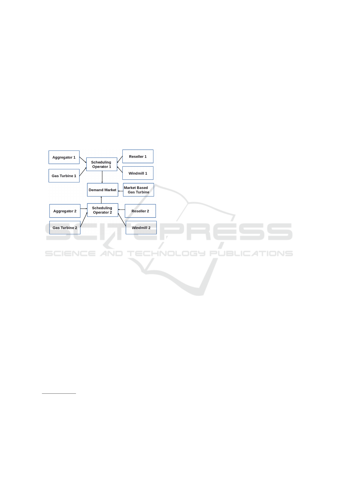
2 PROBLEM STATEMENT
Figure 1 represents the micro grid model which we
study. Here, a scheduling operator, an aggregator,
a reseller, and a windmill form a coalition and two
such coalitions interact with each other through the
demand market. We have simulated an hour ahead
scenario of energy exchanges where both demand and
production is flexible (i.e. adaptive to tariff) and com-
pared it to the non flexible case. We formulated the
situation as an optimizing problem, solving which
gives optimal tariffs for the distributors and allows to
assess the impact of flexibility in both energy savings
and revenue maximization.
Figure 1: Interaction model among various actors of the
micro grid.
3 MODELING OF THE
PRODUCER
In this study, it is assumed that an electricity producer
is either dealing with one and only one scheduling op-
erator or directly selling energy on the demand mar-
ket. Further, producer is a role corresponding to only
one production means
1
. In this study, only windmills
and gas turbines are taken into consideration.
3.1 Windmill
Since we are interested in an hourly interaction be-
tween the coalitions, one time investment costs are
not considered. As thus the windmill is assumed to
produce energy at cost 0. The windmills are always
in contract with a scheduling operator and thus can-
not contribute in the market. The production level of
a windmill is partially uncertain and thus modeled as a
1
There exist many production means: windmill, photo-
voltaic plant, hydro-power plant (over water, or in moun-
tains), gas turbine, nuclear plants to name a few.
random process. E
wm
is the hourly energy production
expectancy calculated on the basis of past history.
3.2 Gas Turbine
A gas turbine sells energy as requested by the
scheduling operators or market. Thus, it charges the
price as per amount of energy produced. Since we
worked with real life data, we used the General Elec-
tric 9E gas turbine series and work of (Roche, 2012)
to model the gas turbine pricing function as given by
Equation (1).
Local Gas Turbine are in contract with a schedul-
ing operator. Therefore, the scheduling operator buys
from its contracted gas turbine before going to the
market to buy extra energy if needed. P
`
gt
(E
`
gt
) denotes
the cost for producing E
`
gt
amount of energy. E
`
max
is
the maximum amount of energy that can be produced
by the local gas turbine.
Market based Gas Turbine are similar to local gas
turbines except they have no capacity constraint and
are connected to the demand market. They have a
higher charge than their local counterparts since they
are not guaranteed to make profit via selling at every
hour. P
m
gt
(E
m
gt
) is the price for selling E
m
gt
amount of
energy. While selling, the market based gas turbine
keeps an additional constant profit margin C
m
> 0 per
unit of energy sold.
P
α
gt
(E
α
gt
) = 0.2(E
α
gt
)
2
+ (143 +C
α
)E
α
gt
+ 6088,
with α ∈ {`, m}, C
`
= 0, E
α
gt
> 0
(1)
4 MODELING OF THE
CONSUMER
We model the consumers and classify them into two
broad groups. Those who are willing to accept a
power offering which is less than the power they de-
manded, in exchange for a monetary compensation
can be thought to draw power from a flexible distrib-
utor. Those with non flexible demand needs like hos-
pitals can be labeled as a separate group who draw
power from a non flexible distributor.
4.1 Reseller
The reseller is an actor in the smart grid, who serves as
a non flexible distributor. It buys energy from the con-
tracted scheduling operator and sells to its customers.
It has no bound on the energy level it can sell.
SMARTGREENS 2016 - 5th International Conference on Smart Cities and Green ICT Systems
352

For a reseller, T
r
is the price per unit of energy
at which it buys from the scheduling operator and E
r
is corresponding amount of energy bought. C
r
is the
effective cost to the reseller and is given by C
r
= E
r
T
r
.
4.2 Aggregator
An aggregator is in business with a scheduling opera-
tor and behaves as a flexible distributor. It has its own
customers with their energy needs. The distinguish-
ing role of an aggregator (compared to a reseller) is
that it can influence its customers to reduce their en-
ergy needs with price incentives.
4.2.1 Flexibility Curve for Aggregator
Let us define the allotted energy ratio for the aggrega-
tor as
E
∗
a
=
E
a
E
da
,
where E
a
and E
da
represent the energy allotted to the
aggregator and actual demand of the aggregator re-
spectively. The minimum allotted energy ratio that
has to be provided is
E
∗
min,a
=
E
min,a
E
da
,
where E
min,a
is the minimum energy that has to be
consumed by aggregator even at infinite cost. E
∗
a
may
be time varying while E
∗
min,a
is kept constant and is
fixed at 0.7. E
∗
min,a
can be also made time varying so
as to decrease it during hours of high requirement and
increase in the opposite case.
Let T
a
be the tariff charged to the aggregator. The
tariff of the aggregator can be modeled by:
T
∗
=
T
a
T
r
.
The relation between E
∗
a
and T
∗
is given by a lin-
ear flexibility function
φ(T
a
) = 1 −
T
a
T
r
= 1 − T
∗
.
The proposed linear function for energy bought by
aggregator is
E
∗
a
= φ(T
a
)+(1−φ(T
a
))E
∗
min,a
, with T
a
∈ [0, T
r
]. (2)
Equation (2) expresses the fact as T
∗
decreases, the
energy satisfaction increases while at a higher tariff
lower energy is consumed by the aggregator. Thus a
flexibility is observed with respect to tariff charged to
the aggregator.
Simplifying the algebra, the energy bought by ag-
gregator E
a
can finally be written
E
a
= E
da
1 − (1 − E
∗
min,a
)T
∗
, with T
∗
∈ [0,1].
The effective price charged by the scheduling
operator can then be calculated by multiplying the
amount of energy sold by per per unit price:
C
a
(E
∗
a
) = T
a
E
a
= E
da
E
∗
a
T
r
1 − E
∗
a
1 − E
∗
min,a
. (3)
4.2.2 Compensation Function
Although selected through trial and error, the ratio-
nale behind a compensation function is that the com-
pensation tariff should be more than the buying tar-
iff. Consequently, the larger the unsatisfied energy,
the larger the penalty incurred. The sample function
which is used for this model is given by
F
c
(E
∗
a
) = (1 − E
∗
a
)E
∗
da
T
r
log(T
r
). (4)
5 DEFINING THE SCHEDULING
OPERATOR
A scheduling operator is an actor connected with sev-
eral electricity producers and one or several electricity
distributors. Its responsibility is to equilibrate produc-
tion with consumption. If the suppliers, with whom it
is dealing with, cannot provide enough energy, it can
buy electricity on the demand market. Reciprocally, if
the consumption is lower than the production, it can
sell excess energy on the market.
5.1 Market Strategy
Each scheduling operator needs to develop an expec-
tation of market demand per hour. In addition to that,
it needs to formulate its buying and selling valuation
functions for E
x
, the energy in exchange with the mar-
ket. The convention is E
x
> 0 if the scheduling opera-
tor buys from the market and E
x
< 0 if the scheduling
operator sells to the market. Underlying the energy
exchange, lies the energy conservation law, which can
be formulated in our case by
E
wm
+ E
`
gt
+ E
x
= E
r
+ E
a
. (5)
Selling to the Market. The selling price for |E
x
|
amount of energy comes from the difference of pro-
duction cost for total amount of energy generated by
the local gas turbine given by E
gt
and the production
cost for the supply of energy supplied to the aggrega-
tor and reseller which is E
gt
+ E
x
− E
wm
. The selling
price is of the same sign as E
x
, and therefore non pos-
itive by convention and its absolute value is the excess
cost for producing |E
x
|:
P
s,m
(E
x
) = P
l,gt
(E
`
gt
) − P
`
gt
(E
`
gt
− E
x
). (6)
Economical Analysis of Flexibility in Micro Grids
353

Buying from the Market. An amount E
x
of energy
can be bought either (i) from a selling scheduling op-
erator or (ii) from the market gas turbine or (iii) a con-
tribution from both. So the buying price estimation of
a scheduling operator is taken in between the expected
selling price of that amount by the other scheduling
operator and by the market-based gas turbine:
P
b,m
(E
x
) = (γ − 1)P
s,m
(E
x
) + γP
m,gt
(E
x
). (7)
where γ is a parameter between 0 and 1. A high
value of γ signifies that the energy is more likely to
come from the market gas turbine, while a lower value
denotes likeliness to come from the selling schedul-
ing operator. Since the pricing function of the other
scheduling operator for |E
x
| amount of energy is un-
known, we assume each scheduling operator expects
the other to value |E
x
|, the same way it would have.
Thus the expected market function is given by
P
m
(E
x
) =
P
s,m
(E
x
) if E
x
< 0,
P
b,m
(E
x
) otherwise.
(8)
Finally, the value of γ is learned through past ex-
periences.
5.2 Utility / Profit for the Scheduling
Operator
Utility U represents the profit made by any scheduling
operator. It is formulated as the revenue obtained in
selling to the aggregator and the reseller minus the
production cost from the local gas turbine, buying
cost from the market, and the compensation to the ag-
gregator:
U(E
∗
a
,E
x
,E
`
gt
) = C
r
+C
a
(E
∗
a
) − P
m
(E
x
)
−P
l,gt
(E
`
gt
) − F
c
(E
∗
a
).
(9)
Note that with the previous conventions P
m
(E
x
) is
non negative if the scheduling operator is buying en-
ergy from the market and non positive otherwise. The
strategy of the scheduling operator (SO) is then:
max
E
∗
a
,E
x
,E
`
gt
U s.t.
E
wm
+ E
`
gt
+ E
x
= E
r
+ E
∗
a
E
da
,
E
∗
a
∈ [E
∗
min,a
,1],
E
`
gt
∈ [0,E
`
max
].
(10)
The demand market (presented below) has the
property to always allocate the demanded amount to
the buying SO (i.e. those with E
x
> 0) while satisfy-
ing partly or totally the selling SO: that is the amount
to be sold is |
e
E
x
| ≤ |E
x
| if E
x
< 0. Hence, for both
SO, the optimization (10) is solved before entering the
market. Then, for the selling SO, optimization (10) is
solved again after the allocation of the market, with
the extra constraint that for that SO with E
x
=
e
E
x
.
6 MODELING THE DEMAND
MARKET
At the start of each hour, the two scheduling operators
report to the market their willingness to either sell or
buy energy. Three cases can arise:
Buying and Selling Scheduling Operator.
Scheduling operator 1 wants to buy E
1
x
> 0 amount
of energy while scheduling operator 2 wants to sell
E
2
x
< 0. Thus scheduling operator 2 submits a two
dimensional selling bid of the form hE
2
x
,P
2
x
i. The
market computes prices P
A
and P
B
according to:
P
A
= P
2
x
× min
E
1
x
|E
2
x
|
,1
+ P
m
gt
max
0,E
1
x
− |E
2
x
|
,
P
B
= P
m
gt
(E
1
x
).
The buyer gets the amount E
1
x
of energy (as ex-
pected) and is charged P
1
x
= min{P
A
,P
B
}. If P
B
< P
A
,
then the seller gets
e
P
x
2
= 0 and the market gas turbine
receives P
B
. Otherwise, the selling scheduling opera-
tor sells the amount of energy
f
E
2
x
= min
E
1
x
|E
2
x
|
,1
×E
2
x
at total price
f
P
2
x
= min(
E
1
x
|E
2
x
|
,1) × P
2
x
.
Buying Scheduling Operators Only. Let the buy-
ing scheduling operators report their demand E
1
x
and
E
2
x
. The market fetches the total demand of E
1
x
+
E
2
x
from the market based gas turbine at a price of
P
m,gt
(E
1
x
+ E
2
x
) and the buyers are charged a payment
proportional to the energy they requested for.
Selling Scheduling Operators Only. When both
scheduling operators try to sell, then no energy trans-
action takes place in the market. Thus both the
scheduling operators receive a payment of 0.
7 IMPLEMENTATION
Each scheduling operator plans each hour ahead and
thus saves itself from producing any unused amount
of energy. At each hour of simulation, the schedul-
ing operator gets information on expected amount of
production from the windmill. Information is fed into
the Equation (9) to give out the answers of how much
local gas turbine should produce and also how much
to buy or sell to the market.
Then, the reseller and aggregator attached with a
scheduling operator reports its demand for that hour.
As for the simulation, web service is used to relay
the information to the scheduling operator. Once the
SMARTGREENS 2016 - 5th International Conference on Smart Cities and Green ICT Systems
354
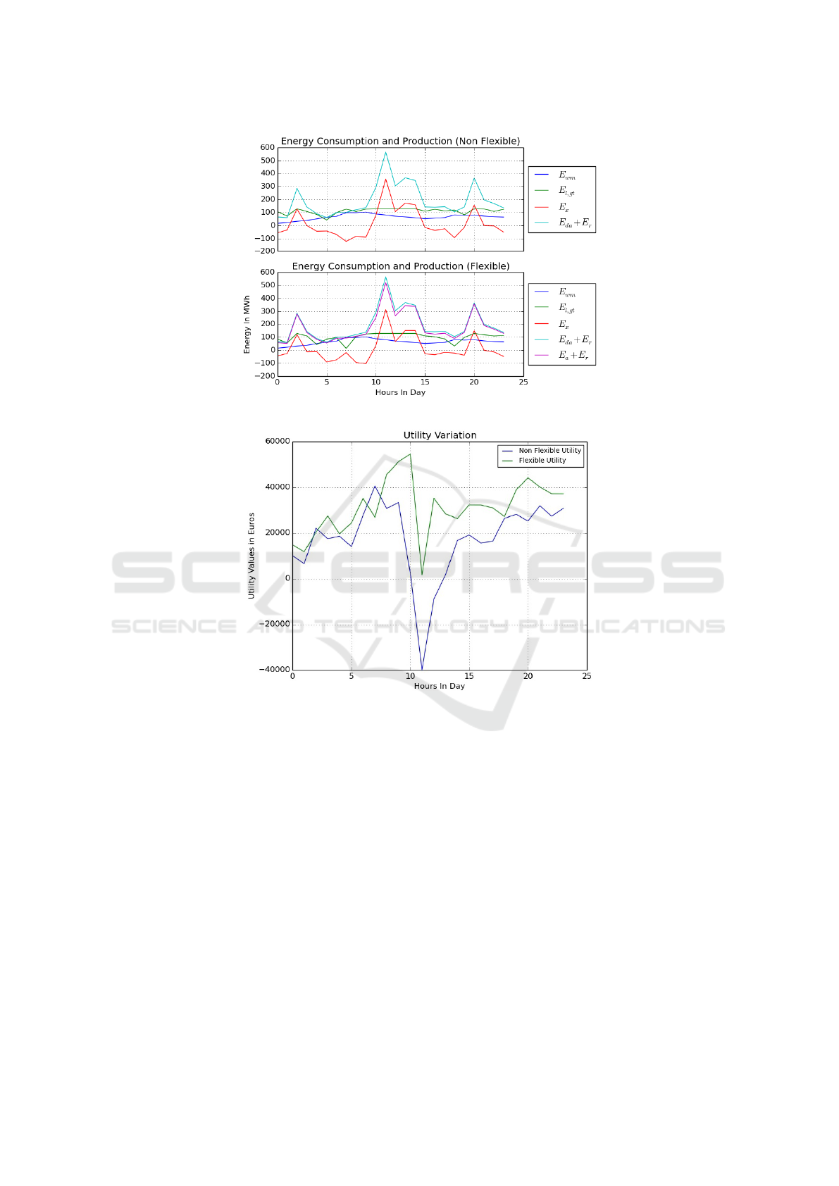
Figure 2: Energy Production and Consumption Comparison.
Figure 3: Utility Value Comparison.
market plays its role, the scheduling operators adjusts
their production and consumption.
The simulation was implemented in Python 3.4
using Flask API on commodity hardware. Each ac-
tor was assigned a server port address and communi-
cation between different actors was carried via HTTP
protocol. The results were later converted into graphs
for visualization using matplotlib.
8 RESULTS AND DISCUSSION
Results can be divided into two parts, the first task
being to find tariff T
r
of each coalition. The second
task is to understand the impact of flexibility on the
smart grid model in terms of profit made.
8.1 Finding Tariff
In order for the optimization to work, we have to set
the tariff for distributors such as aggregators and re-
sellers. Initially, random prices were chosen to see
how the system behaved. It was observed that on set-
ting the tariff too high, the aggregators started behav-
ing like resellers. On lowering the tariff, the schedul-
ing operator on behalf of its coalition made immense
losses. Then, we tried to find the best tariff for each
hour for which there were no losses nor profit for
the scheduling operator, assuming aggregators to be
resellers as well. The average tariff was then cal-
culated over a year. For Scheduling Operator 1 and
Scheduling Operator 2, as given in the model, the tar-
iff came as 300e/MWh and 320e/MWh respectively.
To make the model simple, we have assumed that the
tariffs are time invariant.
Economical Analysis of Flexibility in Micro Grids
355

8.2 Impact of Flexibility
To understand the impact of flexibility, a similar situa-
tion with non flexible operator in one case and flexible
operators on the other must be compared. Here study
has been mainly focused with respect to two parame-
ters namely energy consumption and production and
utility variation. A randomly sampled result has been
put to display.
The plots in Figure 2 show the need of flexibility
in the hours of high demand. It is justified since it is
not wise to trouble the customers all the time as that
might lead to undesirable circumstances. For exam-
ple, in the 11
th
hour, there was an imminent need for
flexibility after the local gas turbine reached its maxi-
mum operating point. The plots in Figure 3 show the
variation of utility/profit in both cases. It can be ob-
served that at the time of flexibility, the non flexible
operator incurred a loss while the flexible one made a
profit, no matter how meager it is. From an econom-
ical standpoint, flexibility resulted in a better utility
than being non flexible keeping the other parameters
constant.
9 CONCLUSION
In this paper, though we have kept the mathematical
modeling simple, the impact of flexibility at aggrega-
tor level have been quite prominent. The naive way of
finding an optimal tariff, seemed effective in showing
flexibility. More importantly, the system showed flex-
ibility only in times of high demand, automatically
modeling the comfort level of the consumers. Find-
ing out the optimal tariff for the system is worth re-
searching as it is one of the critical parameter for the
system to show flexibility. Instead of keeping it con-
stant throughout the day, it can made to vary along
different hours of the day. There is lack of strategies
in the paper, by virtue of which a scheduling operator
can model others. Possible scopes of experimenting
lies in formulation of the flexibility function and com-
pensation function for the aggregator. The interaction
between the scheduling operators via the market can
be thought of as an auction mechanism. Herein lies
the future scope of game theory into modeling the ex-
pectation function for the scheduling operators along
with bidding strategies. With more than two schedul-
ing operators in the market, the grid dynamics will be
interesting to observe.
REFERENCES
Albadi, M. H. and El-Saadany, E. (2007). Demand response
in electricity markets: An overview. In IEEE power
engineering society general meeting, volume 2007,
pages 1–5.
Chen, C., Kishore, S., and Snyder, L. V. (2011). An innova-
tive RTP-based residential power scheduling scheme
for smart grids. In IEEE International Conference on
Acoustics, Speech and Signal Processing (ICASSP),
pages 5956–5959.
Fadlullah, Z. M., Nozaki, Y., Takeuchi, A., and Kato, N.
(2011). A survey of game theoretic approaches in
smart grid. In IEEE International Conference on Wire-
less Communications and Signal Processing (WCSP),
pages 1–4.
Gkatzikis, L., Koutsopoulos, I., and Salonidis, T. (2013).
The role of aggregators in smart grid demand response
markets. IEEE Journal on Selected Areas in Commu-
nications, 31(7):1247–1257.
Maity, I. and Rao, S. (2010). Simulation and pricing mecha-
nism analysis of a solar-powered electrical microgrid.
Systems Journal, 4(3):275–284.
Mohsenian-Rad, A.-H., Wong, V. W., Jatskevich, J., and
Schober, R. (2010a). Optimal and autonomous
incentive-based energy consumption scheduling algo-
rithm for smart grid. In Innovative Smart Grid Tech-
nologies (ISGT), 2010, pages 1–6. IEEE.
Mohsenian-Rad, A.-H., Wong, V. W., Jatskevich, J.,
Schober, R., and Leon-Garcia, A. (2010b). Au-
tonomous demand-side management based on game-
theoretic energy consumption scheduling for the fu-
ture smart grid. IEEE Transactions on Smart Grid,
1(3):320–331.
Momoh, J. et al. (2009). Smart grid design for efficient
and flexible power networks operation and control. In
IEEE/PES Power Systems Conference and Exposition
(PSCE), pages 1–8.
Nguyen, P. H., Kling, W. L., and Ribeiro, P. F. (2013). A
game theory strategy to integrate distributed agent-
based functions in smart grids. IEEE Transactions on
Smart Grid, 4(1):568–576.
Roche, R. (2012). Algorithmes et architectures multi-
agents pour la gestion de l’
´
energie dans les r
´
eseaux
´
electriques intelligents. Application aux centrales
`
a
turbines
`
a gaz et
`
a l’effacement diffus r
´
esidentiel.
PhD thesis, Universit
´
e de Technologie de Belfort-
Montb
´
eliard, Institut de Recherche sur les Trans-
ports, l’Energie et la Soci
´
et
´
e / Laboratoire Syst
`
emes
et Transports.
Saad, W., Han, Z., Poor, H. V., and Bas¸ar, T. (2012). Game-
theoretic methods for the smart grid: An overview
of microgrid systems, demand-side management, and
smart grid communications. Signal Processing Mag-
azine, IEEE, 29(5):86–105.
SMARTGREENS 2016 - 5th International Conference on Smart Cities and Green ICT Systems
356
