
Maritime Traffic Models for Vessel-to-Vessel Distances
Gaspare Galati, Gabriele Pavan, Francesco De Palo and Giuseppe Ragonesi
Department of Electronic Engineering, Tor Vergata University, Rome, Italy
Keywords: Vessel Traffic Model, Radar Visibility, Statistical Analysis, Sea Traffic Model.
Abstract: The maritime traffic is significantly increasing in the recent decades due to its advantageous features related
to costs, delivery rate and environmental compatibility. The Vessel Traffic System (VTS), mainly using radar
and AIS (Automatic Identification System) data, provides ship’s information (identity, location, intention and
so on) but is not able to provide any direct information about the way in which ships are globally positioned,
i.e. randomly distributed or grouped/organized in some way, e.g. following routes. This knowledge can be
useful to estimate the mutual distances among ships and the mean number of surroundings vessels, that is the
number of marine radars in visibility. The AIS data provided by the Italian Coast Guard show a Gamma-like
distribution for the mutual distances whose parameters can be estimated through the Maximum-Likelihood
method. The truncation of the Gamma model is a useful tool to take into account only ships in a relatively
small region. The result is a simple one-parameter distribution able to provide indications about the traffic
topology. The empirical study is confirmed by a theoretical distribution coming from the bi-dimensional
Poisson process with ships being randomly distributed points on the sea surface.
1 INTRODUCTION
Maritime traffic is strictly connected to economic
growth: the international shipping industry is
responsible for delivering about 90% of all trade
worldwide (with 7 to 9 billion of tons loaded per
year), and it is vital for bulk transport of raw material,
oil and gas. The linear regression between the
economic growth of the nations in the Organisation
for Economic Cooperation and Development (OECD)
shows a 4% increase of imports and exports for a 1%
increase in the Gross Domestic Product (GDP). So,
marine transportation is an integral, although
sometimes less visible, part of the global economy.
The marine transportation system includes a
network of specialized vessels, as well as the ports
they visit and transportation infrastructure from
factories to terminals to distribution centres to
markets. Maritime transportation is a necessary
complement to other modes of freight transportation,
and it has the peculiar advantage of lower damaging
emissions. In fact, shipping is emitting about 2.7% of
the global greenhouse gases (GHG) (versus 93.7 % of
road) and its energy consumption is about 1.4%
(versus 2.6% of rail, 13.5% of air, 82.5% of road
transport). For many commodities and trade routes,
there is no direct substitute for waterborne commerce.
On other routes, such as some coastwise or short-sea
shipping or within inland river systems, marine
transportation may provide a substitute for roads and
rail, depending upon cost, time and infrastructure
constraints. Other important marine transportation
activities include passenger transportation (ferries
and cruise ships), national defence, fishing and
resource extraction as well as navigational service,
including tugs.
The number of vessels in the world commercial
fleet is about 110000 (for comparison, the number of
operating commercial planes are is about 19% of this
figure: roughly one commercial plane for five
commercial vessels), 41% are cargo (general cargo,
tankers, bulk/combined vessels, containers vessels),
42% "non-cargo" (fishing, passengers, tug boats etc.)
and 17% military, for a global gross tonnage of the
order of 650 millions (Bosch, et al., 2010). A much
larger number of leisure (or pleasure, recreational)
boats is sailing near the shores: only in the USA, this
fleet is about 70000 vessels between 12 and 20 m and
11000 over 20 m. If we consider also these pleasure
boats, even forgetting the billions of smaller leisure
boats worldwide, the spatial distribution of marine
traffic increases significantly in the areas close to one
or more ports.
Since the marine navigation is a potentially
160
Galati, G., Pavan, G., Palo, F. and Ragonesi, G.
Maritime Traffic Models for Vessel-to-Vessel Distances.
In Proceedings of the International Conference on Vehicle Technology and Intelligent Transport Systems (VEHITS 2016), pages 160-167
ISBN: 978-989-758-185-4
Copyright
c
2016 by SCITEPRESS – Science and Technology Publications, Lda. All rights reserved

dangerous activity for the people involved as well as
for the environment, a more efficient and a more
controlled navigation is required to lower the risks
and to increase the overall maritime safety.
To get these achievements, the Vessel Traffic
Service (VTS) has been introduced by the
International Maritime Organization (IMO) in 1985
and then updated in 1997 with the Resolution
A.857(20). The VTS is a service implemented by a
Competent Authority, designed to improve the safety
and efficiency of vessel traffic and to protect the
environment (IMO, 1997).
Unlike the Air Traffic Control (ATC) which
directs aircrafts through controlled airspace (ICAO,
2001), VTS only provides guidelines for procedures
and manoeuvres in a crowded marine area, as well as
information requested by the crew. Hence, outside the
harbour waters the VTS has no any authority to
impose speed and route to follow which are
demanded to the captain’s decision.
In addition to being a “VTS target”, all ships of
300 gross tonnage (or more) engaged on international
voyages and all cargo ships of 500 gross tonnage (and
upwards) even if not engaged on international
voyages, and finally all passenger ships, are required
to carry on an Automatic Identification System (AIS)
transponder (SOLAS, 2002), (IMO, 2001) capable of
automatically exchange relevant information about
the ship (radio call sign, IMO identification number,
vessel name and type, position, heading, course,
speed, destination, navigational status and more) with
other ships and with coastal stations, providing a kind
of Automatic Dependent Surveillance. The primary
use of AIS is to permit each equipped ship to "see and
be seen" by other ships. Concerning the related radio
link, AIS uses the VHF region: Channel A 161.975
MHz, Channel B 162.025 MHz, with a particular self-
organized time-division multiple access to the radio
channel, for short, SO-TDMA. The maximum
distance in this ship-to-ship radio communication is
limited by propagation over sea of the used waves
and, depending on the environment and VHF antenna
height, it is about 20 nautical miles (one nautical mile
- N.M. or nm or n mi - equals 1852 m), while marine
radars, operating in the microwave region, are
generally propagation-limited to about half this
figure. The aforementioned autonomous operation of
vessels, however, does not help to achieve a well-
organized marine traffic and, based on raw AIS or
radar data, little can be said – in general – about the
overall way in which ships are positioned in a given
area and about the distribution of their mutual
distances. The type of ship, and its destination, are
only available for AIS-equipped vessels, the model
proposed in this paper is aimed to infer some
characteristics of all marine traffic for every type of
vessels, including non-cooperating ones whether they
are VTS or coastal radar targets.
The knowledge of the mutual distances, for
example, can be useful to evaluate the minimum
safety separation as well as, more important from the
scientific point of view, the mean numbers of marine
radars (Briggs, 2004) in visibility that can interfere
with the on-board radar of a given ship (Galati, et al.,
2015). Such visibility results can also be useful to
evaluate the load of the AIS radio channels for
applications such as performance analysis and
installation planning of coastal AIS stations.
In this paper we build up a statistical model of the
mutual distances between pairs of ships focusing on
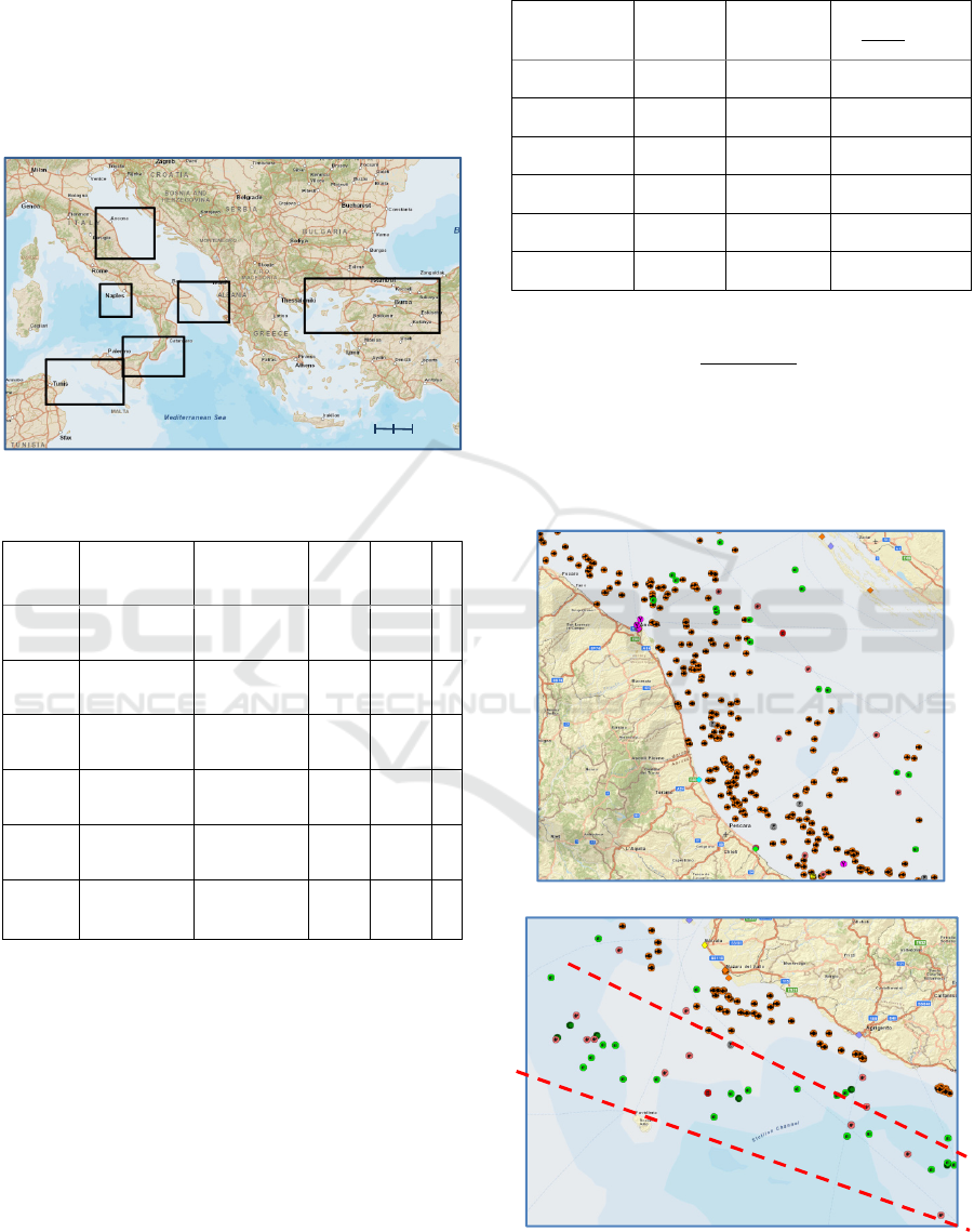
six areas of the Mediterranean sea, see Figure 1. The
model has been derived from real-world AIS data
provided by the Italian Coast Guard for the week Feb
23
th
– Mar 1
st
, 2015. The data analysis has shown that
the mutual distance among ships follows a Gamma-
like statistical distribution. In order to make the model
more general and not AIS-data dependent, we have
estimated the parameters for the empirical Gamma
distribution through the Maximum-Likelihood
estimation. Finally we have considered a conditioned,
i.e. truncated, distribution in order to take into
account the horizon for radar and VHF visibility.
In Chapter 2 the AIS data provided by the Italian
Coast Guard are presented, with the related statistical
analysis in which the parameters of the Gamma and
Generalized Gamma models are estimated.
Chapter 3 considers the truncation of the
distribution of the mutual distances in order to
evaluate the mean number of ships in a given region,
for example for radar applications. A simplified
truncated model with only one parameter has been
developed for the mutual distances. The relationship
between the model parameters and the topology of the
traffic has been investigated. To confirm the
empirical work, a more general theoretical Poisson-
like model has been treated.
2 THE MARINE TRAFFIC
MODEL
In this section the statistical model for the mutual
distances is derived from the AIS data.
2.1 AIS Data and their Distribution
The General Command of the Italian Coast Guard
Maritime Traffic Models for Vessel-to-Vessel Distances
161
kindly provided the AIS data for the week Feb 23
th
–
Mar 1
st
, 2015 related to six areas: (1) Central Adriatic,
(2) Otranto Canal, (3) Central Tyrrhenian, (4)
Messina Strait, (5) Canal of Sicily and (6)
Dardanelles/Bosporus (see Figure 1).
See Table 1a for more details. Each area was
sampled at regular intervals of four hours from
midnight (Galati, et al., 2015), (Galati and Pavan, 2015).
Figure 1: View of the six Mediterranean areas.
Table 1a: Main characteristics of the six areas.
Area
Point N-E
(DMS)
Point S-O
(DMS)
Total
Surface
[nm
2
]
Sea
Surface
[nm
2
]
Sea
[%]
(1) Central
Adriatic
44°10’18.40’’N
15°55’16.71’’E
42°09’26.58’’N
12°43’13.25’’E
22632 13600 60
(2) Otranto
Canal
41°12’57.47’’N
20°01’18.74’’E
39°31’42.97’’N
17°12’28.32’’E
17712 12300 69
(3) Central
T
yrrhenian
41°07’27.98’’N
14°40’34.17’’E
39°46’’07.02’’N
12°55’19.09’’E
8455 6700 79
(4)Messina
Strait
38°55’08.47’’N
17°33’00.99’’E
37°13’27.60’’N
14°10’22.01’’E
20384 13700 67
(5) Canal
of Sicily
37°56’26.98’’N
14°14’01.89’’E
35°59’03.12’’N
09°56’44.44’’E
30186 22800 75
(6)
Dardenelles
Bosporus
41°21’26.79’’N
31°32’03.49’’E
39°05’16.24’’N
24°09’53.99’’E
60112 21700 36
From the first analysis of the AIS data, we derived
the time slot with maximum number of ships in each
area, as shown in Table 1b.
In the following we refer to the area with the
highest traffic as the area with the highest number of
ships.
The density of en-route ships is calculated as the
number of ships over the percentage of sea in the
highest traffic condition.
We extrapolated ships’ positioning information
from the AIS data related to Table 1b (i.e. highest
traffic condition) for each area. We used the flat earth
approximation for distance due to the small-sized
areas (max distance in area (6) is about 370).
Table 1b: Maximum number of ships per each area and their
density . Data for the week Feb 23
th
– Mar 1
st
, 2015.
Area
Day and
Time (in
May, 2015)
Max
number
of ships, N
Ships’ density
×
(1) Central
Adriatic
Tue 24
th
04:00
285 20.88
(2) Otranto
Canal
Tue 24
th
08:00
46 3.74
(3) Central
Tyrrhenian
Fri 27
th
08:00
45 6.72
(4) Messina
Strait
Fri 27
th
16:00
74 5.40
(5) Canal of
Sicily
Fri 27
th
08:00
104 4.56
(6) Dardenelles
Bosporus
Thu 26
th
12:00
53 2.44
The number of mutual distances is:
=
⋅(−1)
2
(1)
in which is the total number of ships in the area in
a specific time slot (e.g. the highest traffic condition).
It is worth to note that the distances are not
statistically independent because they are “mutual”
Area (1) – Central Adriatic
Area (5) – Canal of Sicily
Figure 2: Distributed traffic of Area (1) Central Adriatic
and in-line traffic of Area (5) Canal of Sicily. The dashed
lines highlight a possible route.
4
3
2
1
5
6
Scale = 1:7M
0 200 km
0 108 nm0 108 nm
VEHITS 2016 - International Conference on Vehicle Technology and Intelligent Transport Systems
162
among ships: given ships, if only one of them is
moved, −1 distances do change.
Figure 2 shows the AIS positions of the vessels
for Central Adriatic and Canal of Sicily.
It is known that the traffic in Central Adriatic is
mainly made of fishing boats (88%) whose positions
are someway randomly distributed, while in the Canal
of Sicily are present cargos (20%) following some
well defined (non random) routes.
2.2 Statistical Analysis of Inter-Ship
Distances
The ship-to-ship distance R can be fitted with a
probability density function
(
)
having the
following properties:
•
(
)
=0,≤0
• lim
→
(
)
=0
A suitable candidate for this positive random
variable is the Gamma model whose parameters may
be related to the density of ships. According to the
performed “Goodness of Fit” analysis the Rayleigh
distribution (or “one parameter” Gamma) does not
provide the best fitting because of the very different
traffic conditions difficult to be modelled with one
parameter. On the other hand, the Gamma density
function (Papoulis, 1990):
(
)
=
(
)
≥0
(2)
where Γ
(
)
=
is the Gamma
function, having two-parameters (i.e. the scale
parameter and the shape parameter ), can be better
matched to the empirical data.
In order to improve the model of the AIS data, a
third parameter can be added in Eq. (2) obtaining a
Generalized Gamma model (Stacy, 1962):
(
)
=
⋅
(
)
(
)
>0
(3)
The quantities , are shape parameters. When
=1 the Generalized Gamma density function
coincides with the Gamma model.
These parameters can be estimated by the
Maximum Likelihood (ML) method, which leads to a
system of non-linear equations whose solutions are the
values shown in Table 2 where the last column (right
side) reports the estimated mean values
(in nm).
The sample size for each area is varying from 990
distances with average value of 32.8 nm (area 3) to
40470 distances with average value of 55.6 nm (area
1); day and time are listed in the above Table 1b.
Table 2: Estimated parameters of the Gamma model (a) and
of the Generalized Gamma model (b) for the six areas.
(a)
Area
Gamma Model
=
[]
/
[
]
×
(1) 2.1542 38.7 55.66 2.66
(2) 1.9371 47.2 41.04
11.0
(3) 2.0472 62.4 32.80 4.88
(4) 2.4059 42.9 56.08 10.4
(5) 1.8674 34.7 53.81 11.8
(6) 1.5753 27.4 57.50 23.5
(b)
Area
Generalized Gamma Model
=
+
[
]
×
(1) 0.6061 2.287 11.9 55.63
(2) 0.8303 1.709 19.1 41.01
(3) 0.3334 3.576 16.5 33.04
(4) 0.3939 3.525 10.6 55.89
(5) 0.3848 3.03 10.3 53.63
(6) 0.7918 1.559 13.1 57.63
For the Gamma model the ratio
gives an idea
about the topology of the traffic on the considered sea
surface (e.g. en-route or randomly distributed): a low
ratio values correspond to a distributed, or random,
topology (i.e. Central Adriatic, Area (1)), while
higher values are related to a route, more regular
topology (for example, in Otranto Canal (2), Messina
Strait (4) and Canal of Sicily (5)).
Moreover we observe that the ML estimation of
leads to a system of three non linear equations where
the µ-th power of the sample values (i.e. the measured
distances) is present. Therefore it is necessary to find
that value of whereby the derivative of the
Likelihood function,
(
)
, is equal to zero (see Figure
3). However, as shown in Figure 3, the values of
(
)
in the field of practical interest, i.e. 0< <3, are
close to zero, i.e. there are sub-optimal solutions
(values of ̂) that can be considered, including ̂=1.
Figure 3: The derivate of the Likelihood function for the
estimation of the Generalized Gamma parameter . The
̂
is obtained posing
(
)
=0.
0.5 1 1.5 2 2.5 3 3.5 4
-0.05
-0.04
-0.03
-0.02
-0.01
0
0.01
0.02
f(
μ
)
μ
Area (1)
Area (2)
Area (3)
Area (4)
Area (5)
Area (6)
Maritime Traffic Models for Vessel-to-Vessel Distances
163
The use of ̂=1 simplifies the model leading
back to the Gamma model that looks more convenient
than its generalization (see also in the following).
In order to validate the estimated parameters
,
̂
,
the Kolmogorov-Smirnov test and the
test (Papoulis, 1990) should be applied with the null
hypothesis being (resp. for the Gamma and the
Generalized Gamma distribution):
:
(
)
=
(
)
or
:
(
)
=
(
)
However, since the distances are not
independent, the tests reject too often the null
hypothesis
(Gleser & Moore, 1983), and cannot be
effectively applied in the present case. However, a
visual inspection gives a fairly good idea of the
goodness of fit of the measures mutual distances with
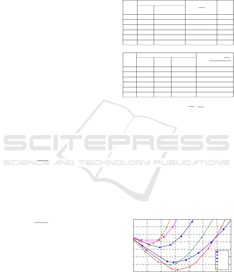
these distribution. In fact, in Figure 4a-f the
histograms of distances for all areas are presented
with the overlapped Gamma and Generalized Gamma
estimated models.
Figure 4a: Histogram and densities of for Areas (1).
Figure 4b: Histogram and densities of for Areas (2).
Figure 4c: Histogram and densities of for Areas (3).
Figure 4d: Histogram and densities of for Areas (4).
Figure 4e: Histogram and densities of for Areas (5).
Figure 4f: Histogram and densities of for Areas (6).
In some cases, e.g. Areas (3) and (5), the
Generalized Gamma model is not the best fit because
the third parameter improves the fitting only
locally. Hence, the Gamma model with parameters
and will be used in the remaining part of this paper.
3 VISIBILITY
In the previous section we have shown that the
distances between pairs of ships can be modelled with
a random variable distributed according to a
Gamma model with parameters and .
It can be useful to consider, for a generic ship, the
mean number of vessels in the surroundings within a
specific area. This need refers to the VHF
communications as well as to the radar interferences
0 20 40 60 80 100 120 140 160 180
Distance, R (nm)
0
0.002
0.004
0.006
0.008
0.01
0.012
0.014
Histogram: Area (1)
Gamma
Generalized Gamma
Probability Density
Probability Density
Probability Density
VEHITS 2016 - International Conference on Vehicle Technology and Intelligent Transport Systems
164
due to solid-state marine radars on board nearby other
vessels (Galati, et al., 2015). In the radar case the
optical horizon – with the 4/3 earth propagation
model – and the heights of ships must be considered
in order to compute the maximum distance at which
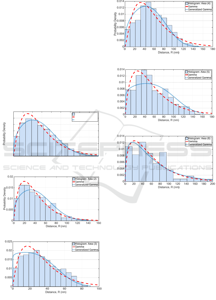
two on-board radars may interfere. This radar horizon
is related to the heights of on-board radars
and
as shown in Figure 5.
Figure 5: Radar visibility between ships and .
In standard atmosphere, making use of the equivalent
earth radius
=
≅8500, the horizon
results:
=
+
≅
2
∙
+
(4)
The antenna height is not included in AIS data,
hence we had empirically estimated the relation
between the length (as provided by AIS) of the ship
and the radar antenna height (Galati, et al., 2015). For
example, if we consider two cargos with their radar
antenna at 30 m above sea level, the optical horizon
is about
=35, while it becomes
=
10 for small and pleasure boats, with antenna
heights of the order of 4 m. In this section we focus
only on the latter case (
=10).
Let’s consider an all-sea circular section with
diameter
. It is possible to calculate the average
number of ships randomly distributed in this circular
sea surface through the probability that the mutual
distances among them should not exceed
:
≤
=
1
Γ()
=(,)
(5)
where (,) is the Incomplete Gamma Function
(Abramowitz & Stegun, 1964) with =⋅
.
The parameters and have been estimated with the
Maximum Likelihood method for each area (Table 2).
Multiplying the probability in Eq. (5) by the total
number of ship in the area
(
)
we obtain the
expected number of ships inside the related area.
=
≤
⋅
(6)
The probability density of the random variable ,
i.e. the mutual distances among the
vessels in
the area (with 0≤≤
) is given by the
conditional density function of Eq. (2):
(
|
≤
)
=
(
)
(
)
0<<
0≥
(7)
This conditional density function can be
computed using the already described and evaluated
Gamma model. This approach uses, for the
conditioned model, the same parameters estimated for
the original model and therefore might be not fully
reliable.
Using Eq. (7) to compute the conditional density
model from the Gamma model with parameters , it
is readily obtained:
(
|
≤
)
=
(,
)
0<<
0≥
(8)
In Eq. (8) we have added the third parameter
named truncation parameter which takes into account
the maximum distance at which the model should be
considered (e.g. the optical horizon).
To estimate and in Eq. (8), having fixed the
value of
, a closed-form solution such as the
well-known one for the Gamma and Generalized
Gamma distribution does not exist. The problem of
finding the maximum for the Likelihood function has
to be solved by a non-linear optimization method. In
particular, we have used the Nelder-Mead algorithm
(Nelder & Mead, 1965).
This estimation often gives very low values for ,
as shown in Table 3 for Areas (1) – (4).
Table 3: Estimation of , , for
=10.
Area
Truncated Gamma
Truncated Generalized
Gamma
[
]
[
]
(1) 1.46
9.3×10
1.46 1
9.5×10
(2) 1.58
2.7×10
1.59 1
2.7×10
(3) 1.25
3.6×10
1.26 1
3.7×10
(4) 1.02 0.012 0.19 5.25
6.9×10
(5) 0.99 0.017 1.21 0.82 0.015
(6) 1.74 0.078 0.22 7.10 0.09
Therefore, a different model with →0 has been
considered for the “short range” (i.e. <
,
having set
=10) distance between a pair of
vessels.
If →0 in Eq. (8), the only remaining term is
multiplied by a constant depending on .
Posing =−1 we obtain:
(
|
≤
)
=⋅
(9)
Maritime Traffic Models for Vessel-to-Vessel Distances
165
The unity area condition for Eq. (9) leads to:
⋅
=1 ⟹=
+1
(10)
Therefore, the conditional density function for
truncated distances with a single parameter is:
(
|
≤
)
=
+1
⋅
0<<
0≥
(11)
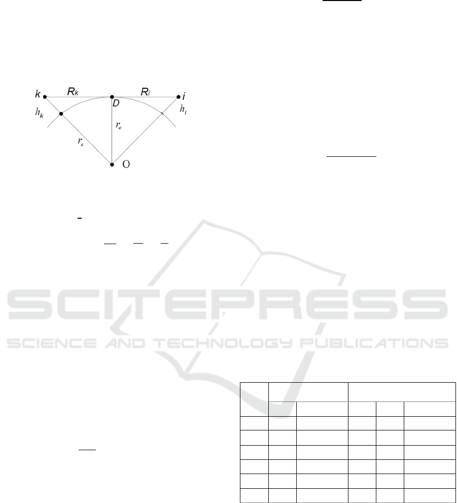
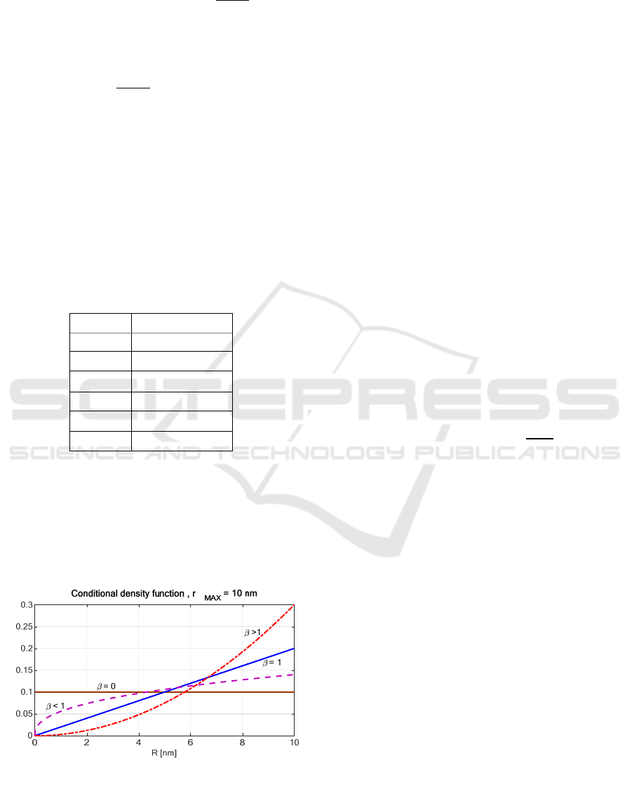
Figure 6 shows Eq. (11) for different values of
(=0,=1,<1 and >1) with
=10.
If →0 (cfr. Table 3) the Gamma model leads to
Eq. (11) and, if ≅0 (cfr. Table 4), the model
converges to the uniform distribution in (0,
) as
shown in Figure 6.
For the six marine areas the ML estimation of the
parameter is shown in Table 4 with
=10.
Table 4: Estimation of for
=10.
Area
(1) 0.461
(2) 0.589
(3) 0.257
(4)
1.95×10
(5)
6.1×10
(6) 0.455
From Table 4 we can find very low values for
in areas (4) and (5), those where the traffic is strongly
channelized. This suggests that strongly channelized
areas generally correspond to low . In fact if the
ships are placed in line, the mean value of the mutual
distances increases making less sharp the slope of the
density function for low values of R.
Figure 6: Conditional density model
(
|
≤
)
for
=0,=1,<1and >1with
=10.
Figure 2 shows the traffic condition for the
Central Adriatic and the Canal of Sicily, the former
with greater than the latter because of the more
randomly distributed vessels in Central Adriatic, as
previously noticed.
It is worth to note that in area (6) is comparable
with the one in Central Adriatic although the area
provides a main route. This effect is due to the
presence in area (6) of two different seas (Aegen and
Sea of Marmara) as well as of Dardanelles, one of the
world's narrowest strait used for international
navigation, with the likely effect of strongly
distorting the behaviour of ships’ distances with
respect to the open sea. In general, the sea percentage
in Table 1 also gives an idea about the reliability of
the values.
3.1 General Poisson’s Model
To corroborate the results we considered another
theoretical model for marine traffic starting from the
bi-dimensional Poisson distribution in which the
ships are placed uniformly in a square with side .
Conditioning the maximum distance to
(with
≪) we obtained the conditional density of
for 0<<
whose limit for →∞ is shown in
Eq. (12) (details are not shown here for the sake of
brevity):
lim
→
(
|
<
)
=
2
(12)
Such a limit represents the condition for which the
range of distances we are interested is much less than
, as in the previous paragraph where
=
10≪≈200.
The limit found in Eq. (12) represents the traffic
uniformly distributed in a interval with edge
≪
, that is the case of =1 in Eq. (11).
If →1 the traffic is Poisson distributed, if →
0 there is a kind of traffic regularity possibly due to
one or more routes. In Table 4 the values of do not
reach the unity because the land imposes a constraint
to the positions, hence on the distances.
The case of >1 is not realistic for marine traffic
since it imposes a mandatory minimal distance among
ships as shown in Figure 6 where the density for low
value is almost zero. This case may be useful to model
other situations such as, possibly, the air traffic.
4 CONCLUSIONS
The empirical analysis of the AIS data has led to a
Gamma model for the mutual distances among ships,
f(r|R < r
MAX
)
VEHITS 2016 - International Conference on Vehicle Technology and Intelligent Transport Systems
166

with the Generalized Gamma model being not the
best solution to fit the data. We estimated the
parameters of the models through the ML method.
Considering the application related to the
interferences between marine (navigation) solid-state
radars, we have truncated the Gamma model to a
maximum distance
in order to take into account
only the ships inside the horizon.
The truncation has led to a more convenient one-
parameter distribution whose parameter is related
to the topology of the traffic in the area of interest.
The relation between and the traffic topology
has been confirmed, at a very first extent, by the study
of a general Poisson model with only one-parameter,
that is , in addition to the truncation limit
.
ACKNOWLEDGEMENTS
Special thanks are due to to C.V. Giuseppe Aulicino
and to S.T.V. Antonio Vollero of the Italian Coast
Guard for kindly providing AIS data of traffic.
REFERENCES
Abramowitz, M. & Stegun, I. A., 1964. Handbook of
mathematical functions. New York: Dover
Publications.
Bosch, T. et al., 2010. World Ocean Review. Hamburg:
Maribus.
Briggs, J. N., 2004. Target Detection By Marine Radar.
London: The Institution of Electrical Engineers.
Galati, G. & Pavan, G., 2015. Mutual interference problems
related to the evolution of marine radars. Las Palmas,
Gran Canaria (Spain), Intelligent Transportation
Systems (ITSC), IEEE, pp. 1785-1790.
Galati, G., Pavan, G. & De Palo, F., 2015. Interference
problems expected when solid-state marine radars will
come into widespread use. Salamanca (Spain), IEEE,
pp. 1-6.
Gleser, L. J. & Moore, D. S., 1983. The effect of
dependence on chi-squared and empiric distribution
tests of fit. The Annals of Statistics, 11(4), pp. 1100-
1108.
ICAO, 2001. Air Traffic Service - Air Traffic Control
Service, Flight Information Service, Alerting Service.
13th ed. : ICAO.
IMO, 1997. Resolution A.857(20) - Guidelines for Vessel
Traffic Services.
IMO, 2001. Resolution A.917(22) - Guidelines for the
onboard operational use of shipborne automatic
identification systems (AIS).
Nelder, J. A. & Mead, R., 1965. A simplex method for
function minimization. The computer Journal, 7(4), pp.
308-313.
Papoulis, A., 1990. Probability and statistics. : Prentice-
Hall.
SOLAS, 2002. Regulation 19 of SOLAS Chapter V -
Carriage requirements for shipborne navigational
systems and equipment.
Stacy, E. W., 1962. A generalization of the gamma
distribution. The Annals of Mathematical Statistics,
September, Volume 33, pp. 1187-1192.
Maritime Traffic Models for Vessel-to-Vessel Distances
167
