MR-SAT: A MapReduce Algorithm for Big Data Sentiment Analysis on

Twitter

Nikolaos Nodarakis

, Spyros Sioutas

, Athanasios K. Tsakalidis

and Giannis Tzimas

Computer Engineering and Informatics Department, University of Patras, 26504 Patras, Greece

Department of Informatics, Ionian University, 49100 Gorfu, Greece

Computer & Informatics Engineering Department, Technological Educational Institute of Western Greece,

26334 Patras, Greece

Keywords:

Big Data, Bloom Filters, Classiﬁcation, MapReduce, Hadoop, Sentiment Analysis, Twitter.

Abstract:

Sentiment analysis on Twitter data has attracted much attention recently. People tend to express their feelings

freely, which makes Twitter an ideal source for accumulating a vast amount of opinions towards a wide diver-

sity of topics. In this paper, we develop a novel method to harvest sentiment knowledge in the MapReduce

framework. Our algorithm exploits the hashtags and emoticons inside a tweet, as sentiment labels, and pro-

ceeds to a classiﬁcation procedure of diverse sentiment types in a parallel and distributed manner. Moreover,

we utilize Bloom ﬁlters to compact the storage size of intermediate data and boost the performance of our

algorithm. Through an extensive experimental evaluation, we prove that our solution is efﬁcient, robust and

scalable and conﬁrm the quality of our sentiment identiﬁcation.

1 INTRODUCTION

Twitter is one of the most popular social network web-

sites and launched in 2006. It is a wide spreading

instant messaging platform and people use it to get

informed about world news, videos that have become

viral, etc. Inevitably, a cluster of different opinions,

that carry rich sentiment information and concern a

variety of entities or topics, is formed. Sentiment is

deﬁned as ”A thought, view, or attitude, especially

one based mainly on emotion instead of reason”

and

describes someone’s mood or judge towards a speciﬁc

entity. User-generated content that captures sentiment

information has proved to be valuable and its use is

widespread among many internet applications and in-

formation systems, such as search engines.

Hashtags are a convention for adding additional

context and metadata to tweets. They are created

by users as a way to categorize their message and/or

highlight a topic and are extensively utilized in tweets

(Wang et al., 2011). Moreover, they provide the abil-

ity to people to search tweets that refer to a com-

mon subject. The creation of a hashtag is achieved

by preﬁxing a word with a hash symbol (e.g. #love).

Emoticon refers to a digital icon or a sequence of key-

http://www.thefreedictionary.com/sentiment

board symbols that serves to represent a facial expres-

sion, as

:-)

for a smiling face

. Both, hashtags and

emoticons, provide a ﬁne-grained sentiment learning

at tweet level which makes them suitable to be lever-

aged for opinion mining.

Although the problem of sentiment analysis has

been studied extensively during recent years, existing

solutions suffer from certain limitations. One prob-

lem is that the majority of approaches is bounded in

centralized environments. Moreover, sentiment anal-

ysis is based on, it terms of methodology, natural

language processing techniques and machine learn-

ing approaches. However, this kind of techniques

are time-consuming and spare many computational

resources. Consequently, at most a few thousand

records can be processed by such techniques without

exceeding the capabilities of a single server (Agar-

wal et al., 2011; Davidov et al., 2010; Jiang et al.,

2011; Wang et al., 2011). Since millions of tweets are

published daily on Twitter, it is more than clear that

underline solutions are not sufﬁcient. Consequently,

high scalable implementations are required in order to

acquire a much better overview of sentiment tendency

towards a topic.

In this paper, we propose MR-SAT: a novel

http://dictionary.reference.com/browse/emoticon

140

Nodarakis, N., Sioutas, S., Tsakalidis, A. and Tzimas, G.

MR-SAT: A MapReduce Algorithm for Big Data Sentiment Analysis on Twitter.

In Proceedings of the 12th International Conference on Web Information Systems and Technologies (WEBIST 2016) - Volume 1, pages 140-147

ISBN: 978-989-758-186-1

MapReduce Algorithm for Big Data Sentiment

Analysis on Twitter implemented in Hadoop (White,

2012), the open source MapReduce implementation

(Dean and Ghemawat, 2004). Our algorithm exploits

the hashtags and emoticons inside a tweet, as senti-

ment labels, in order to avoid the time-intensive man-

ual annotation task. After that, we build the feature

vectors of training and test set and proceed to a clas-

siﬁcation procedure in a fully distributed manner us-

ing an AkNN query. Additionally, we encode features

using Bloom ﬁlters to compress the storage space of

the feature vectors. Through an extensive experimen-

tal evaluation we prove that our solution is efﬁcient,

robust and scalable and conﬁrm the quality of our sen-

timent identiﬁcation.

The rest of the paper is organized as follows: in

Section 2 we discuss related work and in Section 3 we

present how our algorithm works. After that, we pro-

ceed to the experimental evaluation of our approach in

Section 4, while in Section 5 we conclude the paper

and present future steps.

2 RELATED WORK

Early opinion mining studies focus on document level

sentiment analysis concerning movie or product re-

views (Hu and Liu, 2004; Zhuang et al., 2006) and

posts published on webpages or blogs (Zhang et al.,

2007). Respectively, many efforts have been made to-

wards the sentence level sentiment analysis (Wilson

et al., 2009; Yu and Hatzivassiloglou, 2003) which

examines phrases and assigns to each one of them a

sentiment polarity (positive, negative, neutral).

Many researchers confront the problem of sen-

timent analysis by applying machine learning ap-

proaches and/or natural language processing tech-

niques. In (Pang et al., 2002), the authors em-

ploy three machine learning techniques to classify

movie reviews as positive or negative. On the other

hand, the authors in (Nasukawa and Yi, 2003) in-

vestigate the proper identiﬁcation of semantic rela-

tionships between the sentiment expressions and the

subject within online articles. Moreover, the method

described in (Ding and Liu, 2007) proposes a set of

linguistic rules together with a new opinion aggrega-

tion function to detect sentiment orientations in online

product reviews.

Nowadays, Twitter has received much attention

for sentiment analysis, as it provides a source of mas-

sive user-generated content that captures a wide as-

pect of published opinions. In (Barbosa and Feng,

2010), the authors propose a 2-step classiﬁer that sep-

arates messages as subjective and objective, and fur-

ther distinguishes the subjective tweets as positive or

negative. The approach in (Davidov et al., 2010) ex-

ploits the hashtags and smileys in tweets and evaluate

the contribution of different features (e.g. unigrams)

together with a kNN classiﬁer. In this paper, we adopt

this approach and create a parallel and distributed ver-

sion of the algorithm for large scale Twitter data. A

three-step classiﬁer is proposed in (Jiang et al., 2011)

that follows a target-dependent sentiment classiﬁca-

tion strategy. Moreover, the authors in (Wang et al.,

2011) perform a topic sentiment analysis in Twitter

data through a graph-based model. A more recent ap-

proach (Yamamoto et al., 2014), investigates the role

of emoticons for multidimensional sentiment analysis

of Twitter by constructing a sentiment and emoticon

lexicon. A large scale solution is presented in (Khuc

et al., 2012) where the authors build a sentiment lexi-

con and classify tweets using a MapReduce algorithm

and a distributed database model. Although the classi-

ﬁcation performance is quite good, the construction of

sentiment lexicon needs a lot of time. Our approach is

much simpler and, to our best knowledge, we are the

ﬁrst to present a robust large scale approach for opin-

ion mining on Twitter data without the need of build-

ing a sentiment lexicon or proceeding to any manual

data annotation.

3 MR-SAT APPROACH

Assume a set of hashtags H = {h

,...,h

} and

a set of emoticons E = {em

,em

,...,em

} associ-

ated with a set of tweets T = {t

,...,t

} (training

set). Each t ∈ T carries only one sentiment label

from L = H ∪ E. This means that tweets contain-

ing more that one labels from L are not candidates

for T, since their sentiment tendency may be vague.

However, there is no limitation in the number of hash-

tags or emoticons a tweet can contain, as long as they

are non-conﬂicting with L. Given a set of unlabelled

tweets TT = {tt

,tt

,...,tt

} (test set), we aim to in-

fer the sentiment polarities p = {p

, p

,..., p

} for

TT, where p

∈ L ∪ {neu} and neu means that the

tweet carries no sentiment information. We build a

tweet-level classiﬁer C and adopt a kNN strategy to

decide the sentiment tendency ∀tt ∈ TT. We imple-

ment C by adapting an existing MapReduce classiﬁ-

cation algorithm based on AkNN queries (Nodarakis

et al., 2014), as described in Subsection 3.3.

3.1 Feature Description

In this subsection, we present in detail the features

used in order to build classiﬁer C. For each tweet we

MR-SAT: A MapReduce Algorithm for Big Data Sentiment Analysis on Twitter

141

combine its features in one feature vector. We apply

the features proposed in (Davidov et al., 2010) with

some necessary modiﬁcations to avoid the production

of an exceeding amount of calculations, thus boosting

the running performance of our algorithm.

3.1.1 Word and N-Gram Features

We treat each word in a tweet as a binary feature. Re-

spectively, we consider 2-5 consecutive words in a

sentence as a binary n-gram feature. If f is a word

or n-gram feature, then

count( f)

(1)

is the weight of f in the feature vector, N

is the num-

ber of times f appear in the tweet and count( f ) de-

clares the count of f in the Twitter corpus. Conse-

quently, rare words and n-grams have a higher weight

than common words and have a greater effect on

the classiﬁcation task. Moreover, we consider se-

quences of two or more punctuation symbols as word

features. Unlike what authors propose in (Davidov

et al., 2010), we do not include the substituted meta-

words for URLs, references and hashtags (URL, REF

and TAG respectively) as word features (see and Sec-

tion 4). Also, the common word RT, which means

”retweet”, does not constitute a feature. The reason

for omission of these words from the feature list lies

in the fact that they appear in the majority of tweets

inside the dataset. So, their contribution as features

is negligible, whilst they lead to a great computation

burden during the classiﬁcation task.

3.1.2 Pattern Features

This is the main feature type and we apply the pattern

deﬁnitions given in (Davidov and Rappoport, 2006)

for automated pattern extractions. We classify words

into three categories: high-frequency words (HFWs),

content words (CWs) and regular words (RWs). A

word whose corpus frequency is more (less) than F

) is considered to be a HFW (CW). The rest of

the words are characterized as RWs. In addition, we

treat as HFWs all consecutive sequences of punctu-

ation characters as well as URL, REF, TAG and RT

meta-words for pattern extraction. We deﬁne a pat-

tern as an ordered sequence of HFWs and slots for

content words. The upper bound for F

is set to 1000

words per million and the lower bound for F

is set

to 10 words per million. Observe that the F

and F

bounds allow overlap between some HFWs and CWs.

To address this issue, we follow a simple strategy as

described next. Assume fr is the frequency of a word

in the corpus; if fr ∈





the word is clas-

siﬁed as HFW, else if fr ∈



the word is

classiﬁed as CW.

We seek for patterns containing 2-6 HFWs and 1-

5 slots for CWs. Moreover, we require patterns to

start and to end with a HFW, thus a minimal pattern

is of the form [HFW][CW slot][HFW]. Additionally,

we allow approximate pattern matching in order to

enhance the classiﬁcation performance. Approximate

pattern matching is the same as exact matching, with

the difference that an arbitrary number of RWs can be

inserted between the pattern components. Since the

patterns can be quite long and diverse, exact matches

are not expected in a regular base. So, we permit

approximate matching in order to avoid large sparse

feature vectors. The weight w

of a pattern feature p

is deﬁned as in Equation (1) in case of exact pattern

matching and as

α· N

count(p)

(2)

in case of approximate pattern matching, where α =

0.1 in all experiments.

3.1.3 Punctuation Features

The last feature type is divided into ﬁve generic fea-

tures as follows: 1) tweet length in words, 2) num-

ber of exclamation mark characters in the tweet, 3)

number of question mark characters in the tweet, 4)

number of quotes in the tweet and 5) number of cap-

ital/capitalized words in the tweet. The weight w

a punctuation feature p is deﬁned as

· (M

+ M

)/3

(3)

where N

is the number of times feature p appears

in the tweet, M

is the maximal observed value of

p in the twitter corpus and M

declare the

maximal values for word, n-gram and pattern feature

groups, respectively. So, w

is normalized by averag-

ing the maximal weights of the other feature types.

3.2 Bloom Filter Integration

Bloom ﬁlters are data structures proposed by Bloom

(Bloom, 1970) for checking element membership in

any given set. A Bloom ﬁlter is a bit vector of length

z, where initially all the bits are set to 0. We can map

an element into the domain between 0 and z − 1 of

the Bloom ﬁlter, using q independent hash functions

,hf

,...,hf

. In order to store each element e into

WEBIST 2016 - 12th International Conference on Web Information Systems and Technologies

142

the Bloom ﬁlter, e is encoded using the q hash func-

tions and all bits having index positions hf

(e) for

1 ≤ j ≤ q are set to 1.

Bloom ﬁlters are quite useful and they compress

the storage space needed for the elements, as we can

insert multiple objects inside a single Bloom ﬁlter. In

the context of this work, we employ Bloom ﬁlters to

transform our features to numbers, thus reducing the

space needed to store our feature vectors. More pre-

cisely, instead of storing a feature we store the index

positions in the Bloom ﬁlter that are set to 1. Never-

theless, it is obvious that the usage of Bloom ﬁlters

may impose errors when checking for element mem-

bership, since two different elements may end up hav-

ing exactly the same bits set to 1. The error probabil-

ity is decreased as the number of bits and hash func-

tions used grows. As shown in the experimental eval-

uation, the side effects of Bloom ﬁlters are negligible

and boost the performance of our algorithm.

3.3 kNN Classiﬁcation Algorithm

In order to assign a sentiment label for each tweet in

TT, we apply a kNN strategy. Initially, we build the

feature vectors for all tweets inside the training and

test datasets (F

and F

respectively). Then, for each

feature vector u in F

we ﬁnd all the feature vectors

in V ⊆ F

that share at least one word/n-gram/pattern

feature with u (matching vectors). After that, we cal-

culate the Euclidean distance d(u,v),∀v ∈ V and keep

the k lowest values, thus forming V

⊆ V and each

∈ V

has an assigned sentiment label L

,1 ≤ i ≤ k.

Finally, we assign u the label of the majority of vec-

tors in V

. If no matching vectors exist for u, we as-

sign a ”neutral” label. We build C by adjusting an

already implemented AkNN classiﬁer in MapReduce

to meet the needs of opinion mining problem.

3.4 Algorithmic Description

In this subsection, we describe in detail the senti-

ment classiﬁcation process as implemented in the

Hadoop framework. We adjust an already imple-

mented MapReduce AkNN classiﬁer to meet the

needs of opinion mining problem. Our approach con-

sists of a series of four MapReduce jobs, with each job

providing input to the next one in the chain. These

MapReduce jobs are summarized in the following

subsections

Pseudo-codes are available in a technical report in

http://arxiv.org/abs/1602.01248

3.4.1 Feature Extraction

In this MapReduce job, we extract the features, as de-

scribed in Subsection 3.1, of tweets in T and TT and

calculate their weights. The output of the job is an

inverted index, where the key is the feature itself and

the value is a list of tweets that contain it.

The Map function takes as input the records from

T and TT, extracts the features of tweets. Afterwards,

for each feature it outputs a key-value record, where

the feature itself is the key and the value consists of

the id of the tweet, the class of the tweet and the

number of times the feature appears inside the sen-

tence. The Reduce function receives the key-value

pairs from the Map function and calculates the weight

of a feature in each sentence. Then, it forms a list l

with the format < t

:... :t

>, where t

the id of the i-th tweet, w

is the weight of the feature

for this tweet and c

is its class. For each key-value

pair, the Reduce function outputs a record where the

feature is the key and the value is list l.

3.4.2 Feature Vector Construction

In this step, we build the feature vectors F

and F

needed for the subsequent distance computation pro-

cess. To achieve this, we combine all features of a

tweet into one single vector. Moreover, ∀tt ∈ TT we

generate a list (training) of tweets in T that share at

least one word/n-gram/pattern feature.

Initially, the Map function separates for each fea-

ture f the tweets that contain it into two lists, training

and test respectively. Also, for each f it outputs a

key-value record, where the key is the tweet id that

contains f and the value consists of f and weight of

f. Next, ∀v ∈ test it generates a record where the

key is the id of v and the value is the training list.

The Reduce function gathers key-value pairs with the

same key and builds F

and F

. For each tweet t ∈ T

(tt ∈ TT) it outputs a record where key is the id of t

(tt) and the value is its feature vector (feature vector

together with the training list).

3.4.3 Distance Computation

In MapReduce Job 3, we create pairs of matching vec-

tors between F

and F

and compute their Euclidean

distance.

For each feature vector u ∈ F

, the Map function

outputs all pairs of vectors v in training list of u. The

output key-value record has as key the id of v and the

value consists of the class of v, the id of u and the

u itself. Moreover, the Map function outputs all fea-

ture vectors in F

. The Reduce function concentrates

∀v ∈ F

all matching vectors in F

and computes

MR-SAT: A MapReduce Algorithm for Big Data Sentiment Analysis on Twitter

143

the Euclidean distances between pairs of vectors. The

Reduce function produces key-value pairs where the

key is the id of u and the value comprises of the id of

v, its class and the Euclidean distance d(u,v) between

the vectors.

3.4.4 Sentiment Classiﬁcation

This is the ﬁnal step of our proposed approach. In this

job, we aggregate for all feature vectors u in the test

set, the k vectors with the lowest Euclidean distance

to u, thus forming V

. Then, we assign to u the label

(class) l ∈ L of the majority of V

, or the neu label if

The Map function is very simple and it just dis-

patches the key-values pairs it receives to the Reduce

function. For each feature vector u in the test set, the

Reduce function keeps the k feature vectors with the

lowest distance to u and then estimates the prevailing

sentiment label l (if exists) among these vectors. Fi-

nally, it assigns to u the label l.

4 EXPERIMENTS

In this section, we conduct a series of experiments to

evaluate the performance of our method under many

different perspectives. Our cluster includes 4 comput-

ing nodes (VMs), each one of which has four 2.4GHz

CPU processors, 11.5GB of memory, 45 GB hard

disk and the nodes are connected by 1 gigabit Ether-

net. On each node, we install Ubuntu 14.04 operating

system, Java 1.7.0

51 with a 64-bit Server VM, and

Hadoop 1.2.1.

We evaluate our method using two Twitter

datasets (one for hashtags and one for emoticons) we

have collected through the Twitter Search API

be-

tween November 2014 to August 2015. We have

used four human non-biased judges to create a list

of hashtags and a list emoticons that express strong

sentiment (e.g #bored and

). We performed some

experimentation to exclude from the lists the hash-

tags and emoticons that either were abused by twit-

ter users or returned a very small number of tweets.

We ended up with a list of 13 hashtags and a list of

4 emoticons. We preprocessed the datasets we col-

lected and kept only the English tweets which con-

tained 5 or more proper English words

and do not

contain two or more hashtags or emoticons from the

aforementioned lists. Moreover, during preprocess-

ing we have replaced URL links, hashtags and ref-

https://dev.twitter.com/rest/public/search

To identify the proper English word we used an avail-

able WN-based English dictionary

erences by URL/REF/TAG meta-words as stated in

(Davidov et al., 2010). The ﬁnal hashtags dataset con-

tains 942188 tweets (72476 tweets for each class) and

the ﬁnal emoticons dataset contains 1337508 tweets

(334377 tweets for each class). In both datasets, hash-

tags and emoticons are used as sentiment labels and

for each sentiment label there is an equal amount

of tweets. Finally, in order to produce no-sentiment

datasets we used Sentiment140 API

(Go et al., 2009)

and a dataset which is publicly available

. We fed

the no hashtags/emoticons tweets contained in this

dataset, to the Sentiment140 API and kept the set

of neutral tweets. We produced two no-sentiment

datasets by randomly sampling 72476 and 334377

tweets from the neutral dataset. These datasets are

used for the binary classiﬁcation experiments.

We assess the classiﬁcation performance of our al-

gorithm using the 10-fold cross validation method and

measuring the harmonic f-score. For the Bloom ﬁlter

construction we use 999 bits and 3 hash functions. In

order to avoid a signiﬁcant amount of computations

that greatly affect the running performance of the al-

gorithm, we deﬁne a weight threshold w = 0.005 for

feature inclusion in the feature vectors. In essence,

we eliminate the most frequent words that have no

substantial contribution to the ﬁnal outcome.

4.1 Classiﬁcation Performance

In this subsection we measure the classiﬁcation per-

formance of our solution using the harmonic f-score.

We use two experimental settings, the multi-class

classiﬁcation and the binary classiﬁcation settings.

Under multi-class classiﬁcation we attempt to assign

a single label to each of vectors in the test set. In the

binary classiﬁcation experiments, we classiﬁed a sen-

tence as either appropriate for a particular label or as

not bearing any sentiment. As stated and in (Davidov

et al., 2010), the binary classiﬁcation is a useful ap-

plication and can be used as a ﬁlter that extracts senti-

ment sentences from a corpus for further processing.

We also test how the performance is affected with and

without using Bloom ﬁlters. The value k for the kNN

classiﬁer is equal to 50. The results of the experi-

ments are displayed in Table 1. In case of binary clas-

siﬁcation, the results depict the average score for all

classes.

For multi-class classiﬁcation the results are not

very good but still they are way above the ran-

dom baseline. We also observe that the results with

and without the Bloom ﬁlters are almost the same.

Thus, we deduce that for multi-class classiﬁcation the

http://help.sentiment140.com/api

https://archive.org/details/twitter

cikm 2010

WEBIST 2016 - 12th International Conference on Web Information Systems and Technologies

144

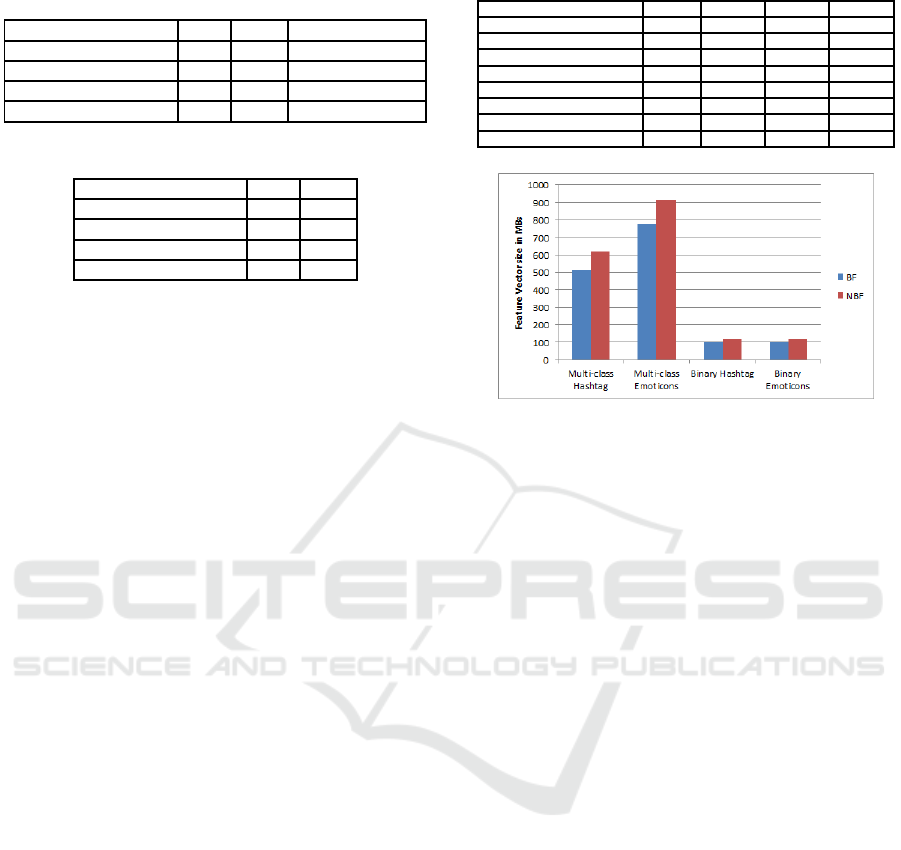
Table 1: Classiﬁcation results for emoticons and hashtags

(BF stands for Bloom ﬁlter and NBF for no Bloom ﬁlter).

Setup BF NBF Random baseline

Multi-class Hashtags 0.32 0.33 0.08

Multi-class Emoticons 0.55 0.56 0.25

Binary Hashtags 0.74 0.53 0.5

Binary Emoticons 0.77 0.69 0.5

Table 2: Fraction of tweets with no matching vectors.

Setup BF NBF

Multi-class Hashtags 0.05 0.01

Multi-class Emoticons 0.05 0.02

Binary Hashtags 0.05 0.03

Binary Emoticons 0.08 0.06

Bloom ﬁlters marginally affect the classiﬁcation per-

formance. Furthermore, the outcome for emoticons

is signiﬁcantly better than hashtags which is expected

due to the lower number of sentiment types. This be-

haviorcan also be explained by the ambiguity of hash-

tags and some overlap of sentiments. In case of binary

classiﬁcation there is a notable difference between the

results with and without Bloom ﬁlters. These results

may be somewhat unexpected but can be explicated

when we take a look in Table 2. Table 2 presents the

fraction of test set tweets that are classiﬁed as neutral

because of the Bloom ﬁlters and/or the weight thresh-

old w (no matching vectors are found). Notice that the

integration of Bloom ﬁlters, leads to a bigger number

of tweets with no matching vectors. Obviously, the

excluded tweets have an immediate effect to the per-

formance of the kNN classiﬁer in case of binary clas-

siﬁcation. This happens since the number of tweets in

the cross fold validation process is noticeably smaller

compared to the multi-class classiﬁcation. Overall,

the results for binary classiﬁcation with Bloom ﬁlters

conﬁrm the usefulness of our approach.

4.2 Effect of k

In this subsection, we attempt to alleviate the problem

of low classiﬁcation performance for binary classiﬁ-

cation without Bloom ﬁlters. To achieve this we mea-

sure the effect of k in the classiﬁcation performance

of the algorithm. We test four different conﬁgurations

where k ∈ {50,100,150, 200}. The outcome of this

experimental evaluation is demonstrated in Table 3.

For both binary and multi-class classiﬁcation, increas-

ing k affects slightly (or not at all) the harmonic f-

score when we embody Bloom ﬁlters. In the contrary

(without Bloom ﬁlters), there is a great enhancement

in the binary classiﬁcation performance for hashtags

and emoticons and a smaller improvement in case of

multi-class classiﬁcation. The inference of this ex-

periment, is that larger values of k can provide a great

Table 3: Effect of k in classiﬁcation performance.

Setup k = 50 k = 100 k = 150 k = 200

Multi-class Hashtags BF 0.32 0.32 0.32 0.32

Multi-class Hashtags NBF 0.33 0.35 0.37 0.37

Multi-class Emoticons BF 0.55 0.55 0.55 0.55

Multi-class Emoticons NBF 0.56 0.58 0.6 0.6

Binary Hashtags BF 0.74 0.75 0.75 0.75

Binary Hashtags NBF 0.53 0.62 0.68 0.72

Binary Emoticons BF 0.77 0.77 0.78 0.78

Binary Emoticons NBF 0.69 0.75 0.78 0.79

Figure 1: Space compression of feature vector.

impulse in the performance of the algorithm when not

using Bloom ﬁlters.

4.3 Space Compression

As stated and above, the Bloom ﬁlters can compact

the space needed to store a set of elements, since more

than one object can be stored to the bit vector. In this

subsection, we elaborate on this aspect and present the

compression ratio in the feature vectors when exploit-

ing Bloom ﬁlters (in the way presented in Section 3.2)

in our framework. The outcome of this measurement

is depicted in Figure 1. In all cases, the Bloom ﬁlters

manage to diminish the storage space required for the

feature vectors by a fraction between 15-20%. Ac-

cording to the analysis made so far, the importance of

Bloom ﬁlters in our solution is twofold. They manage

to both preserve a good classiﬁcation performance,

despite any errors they impose, and compact the stor-

age space of the feature vectors. Consequently, we

deduce that Bloom ﬁlters are very beneﬁcial, when

dealing with large scale sentiment analysis data that

generate an exceeding amount of features.

4.4 Running Time and Scalability

In this ﬁnal experiment, we compare the running time

for multi-class and binary classiﬁcation and measure

the scalability of our approach. Initially, we calculate

the execution time in all cases in order to detect if the

Bloom ﬁlters speedup or slow down the running per-

formance of our algorithm. The results when k = 50

are presented in Figure 2. It is worth noted that in the

MR-SAT: A MapReduce Algorithm for Big Data Sentiment Analysis on Twitter

145

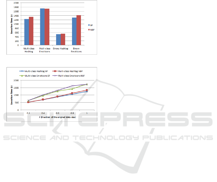
majority of cases, Bloom ﬁlters slightly boost the ex-

ecution time performance. Despite needing more pre-

processing time to produce the features with Bloom

ﬁlters, in the end they pay off since the feature vector

is smaller in size.

Figure 2: Running time.

Figure 3: Scalability.

Finally, we investigate the scalability of our ap-

proach. We test the scalability only for the multi-class

classiﬁcation case since the produced feature vector

in much bigger compared to the binary classiﬁcation

case. We create new chunks smaller in size that are a

fraction F of the original datasets, where F ∈ {0.2,

0.4, 0.6, 0.8}. Moreover, we set the value of k to

50. Figure 3 presents the scalability results of our ap-

proach. From the outcome, we deduce that our algo-

rithm scales almost linearly as the data size increases

in all cases. This proves that our solution is efﬁcient,

robust, scalable and therefore appropriate for big data

sentiment analysis.

5 CONCLUSIONS AND FUTURE

WORK

In the context of this work, we presented a novel

method for sentiment learning in the MapReduce

framework. Our algorithm exploits the hashtags and

emoticons inside a tweet, as sentiment labels, and pro-

ceeds to a classiﬁcation procedure of diverse senti-

ment types in a parallel and distributed manner. Also,

we utilize Bloom ﬁlters to compact the storage size

of intermediate data and boost the performance of our

algorithm. Through an extensive experimental evalu-

ation, we prove that our system is efﬁcient, robust and

scalable.

In the near future, we plan to extend and improve

our framework by exploring more features that may

be added in the feature vector and will increase the

classiﬁcation performance. Furthermore, we wish to

explore more strategies for F

and F

bounds in or-

der to achieve better separation between the HFWs

and CWs. Finally, we plan to implement our solution

in other platforms (e.g. Spark) and compare the per-

formance with the current implementation as well as

other existing solutions, such Naive Bayes or Support

Vector Machines.

REFERENCES

Agarwal, A., Xie, B., Vovsha, I., Rambow, O., and Passon-

neau, R. (2011). Sentiment analysis of twitter data. In

Proceedings of the Workshop on Languages in Social

Media, pages 30–38.

Barbosa, L. and Feng, J. (2010). Robust sentiment detection

on twitter from biased and noisy data. In Proceed-

ings of the 23rd International Conference on Compu-

tational Linguistics: Posters, pages 36–44.

Bloom, B. H. (1970). Space/time trade-offs in hash cod-

ing with allowable errors. Commun. ACM, 13(7):422–

426.

Davidov, D. and Rappoport, A. (2006). Efﬁcient unsuper-

vised discovery of word categories using symmetric

patterns and high frequency words. In Proceedings of

the 21st International Conference on Computational

Linguistics and the 44th Annual Meeting of the As-

sociation for Computational Linguistics, pages 297–

304.

Davidov, D., Tsur, O., and Rappoport, A. (2010). Enhanced

sentiment learning using twitter hashtags and smileys.

In Proceedings of the 23rd International Conference

on Computational Linguistics: Posters, pages 241–

249.

Dean, J. and Ghemawat, S. (2004). Mapreduce: Simpliﬁed

data processing on large clusters. In Proceedings of

the 6th Symposium on Operating Systems Design and

Implementation, pages 137–150.

Ding, X. and Liu, B. (2007). The utility of linguistic rules in

opinion mining. In Proceedings of the 30th Annual In-

ternational ACM SIGIR Conference on Research and

Development in Information Retrieval, pages 811–

812.

Go, A., Bhayani, R., and Huang, L. (2009). Twitter senti-

ment classiﬁcation using distant supervision. Process-

ing, pages 1–6.

Hu, M. and Liu, B. (2004). Mining and summariz-

ing customer reviews. In Proceedings of the Tenth

WEBIST 2016 - 12th International Conference on Web Information Systems and Technologies

146

ACM SIGKDD International Conference on Knowl-

edge Discovery and Data Mining, pages 168–177.

Jiang, L., Yu, M., Zhou, M., Liu, X., and Zhao, T. (2011).

Target-dependent twitter sentiment classiﬁcation. In

Proceedings of the 49th Annual Meeting of the Asso-

ciation for Computational Linguistics: Human Lan-

guage Technologies - Volume 1, pages 151–160.

Khuc, V. N., Shivade, C., Ramnath, R., and Ramanathan, J.

(2012). Towards building large-scale distributed sys-

tems for twitter sentiment analysis. In Proceedings of

the 27th Annual ACM Symposium on Applied Com-

puting, pages 459–464.

Nasukawa, T. and Yi, J. (2003). Sentiment analysis: Cap-

turing favorability using natural language processing.

In Proceedings of the 2Nd International Conference

on Knowledge Capture, pages 70–77.

Nodarakis, N., Pitoura, E., Sioutas, S., Tsakalidis, A. K.,

Tsoumakos, D., and Tzimas, G. (2014). Efﬁcient mul-

tidimensional aknn query processing in the cloud. In

Database and Expert Systems Applications - 25th In-

ternational Conference, DEXA 2014, Munich, Ger-

many, September 1-4, 2014. Proceedings, Part I,

pages 477–491.

Pang, B., Lee, L., and Vaithyanathan, S. (2002). Thumbs

up?: Sentiment classiﬁcation using machine learning

techniques. In Proceedings of the ACL-02 Conference

on Empirical Methods in Natural Language Process-

ing - Volume 10, pages 79–86.

Wang, X., Wei, F., Liu, X., Zhou, M., and Zhang, M. (2011).

Topic sentiment analysis in twitter: A graph-based

hashtag sentiment classiﬁcation approach. In Pro-

ceedings of the 20th ACM International Conference

on Information and Knowledge Management, pages

1031–1040.

White, T. (2012). Hadoop: The Deﬁnitive Guide, 3rd Edi-

tion. O’Reilly Media / Yahoo Press.

Wilson, T., Wiebe, J., and Hoffmann, P. (2009). Recogniz-

ing contextual polarity: An exploration of features for

phrase-level sentiment analysis. Comput. Linguist.,

35(3):399–433.

Yamamoto, Y., Kumamoto, T., and Nadamoto, A. (2014).

Role of emoticons for multidimensional sentiment

analysis of twitter. In Proceedings of the 16th Inter-

national Conference on Information Integration and

Web-based Applications & Services, pages 107–

115.

Yu, H. and Hatzivassiloglou, V. (2003). Towards answering

opinion questions: Separating facts from opinions and

identifying the polarity of opinion sentences. In Pro-

ceedings of the 2003 Conference on Empirical Meth-

ods in Natural Language Processing, pages 129–136.

Zhang, W., Yu, C., and Meng, W. (2007). Opinion retrieval

from blogs. In Proceedings of the Sixteenth ACM Con-

ference on Conference on Information and Knowledge

Management, pages 831–840.

Zhuang, L., Jing, F., and Zhu, X.-Y. (2006). Movie re-

view mining and summarization. In Proceedings of

the 15th ACM International Conference on Informa-

tion and Knowledge Management, pages 43–50.

MR-SAT: A MapReduce Algorithm for Big Data Sentiment Analysis on Twitter

147