Petri Nets Modeling for the Schedulability Analysis of Industrial Real

Time Systems

Alessandro Fantechi and Stefano Pepi

DINFO, University of Florence, Via S. Marta 3, Firenze, Italy

Keywords:

Petri Nets, Timed Petri Nets, Coloured Petri Nets, Real Time Systems, Scheduling Algorithm, Modeling,

Formal Veriﬁcation, Railway Signalling.

Abstract:

In the experience of a railway signaling manufacturer, schedulability analysis takes an important portion of the

time dedicated to conﬁgure a complex, generic, real-time application into a speciﬁcally customized signalling

embedded application. We report on an approach aimed at substituting possibly unreliable and costly empirical

measures with rigorous analysis. The analysis is done resorting to modeling the scheduling algorithms by Petri

Nets. We have compared two types of Petri Nets: Timed Petri Nets (TPN) and Coloured Petri Nets (CPN),

supported by open source tools, respectively TINA and CPN Tools 4.0 concluding that the latter are more

suited for the dealt problem.

1 INTRODUCTION

Real-Time Systems (RTS) are those computer-based

systems where correct operation does not only depend

on the correctness of the results obtained, but also on

the time at which the results are produced (Stankovic,

1988).

The interest for real-time systems is motivated by

many applications that require that computations sat-

isfy given time constraints, in domains such as auto-

motive, avionics, communications, railway signalling

etc.

The most important property of a RTS is pre-

dictability. Predictability is the ability to determine

in advance if the computation will be completed

within the time constraints required. Predictability

depends on several factors, ranging from the archi-

tectural characteristics of the physical machine, to the

mechanisms of the core, up to the programming lan-

guage. Predictability can be measured as the percent-

age of processes for which the constrains are guaran-

teed.

In this article we report the experience made in

collaboration with our industrial partner, a railway

signalling manufacturing company, in the implemen-

tation of a generic real-time platform based on a pro-

prietary microkernel Real Time Operating System;

in particular we present a method for schedulability

analysis.

With the recent expansion of markets to Asia and

Africa, the company has experienced a growing need

for a versatile system that can be conﬁgurable for each

different application. The transition from a traditional

”main loop”-based system to a general purpose plat-

form has allowed low-cost conﬁguration, simply by

changing the application inside and the hardware to

interact with. With the same Hw/Sw platform both

ground and on-board systems can be built, either for

urban (like metro) or main line applications, meeting

the signaling regulations of different countries.

Experience has however shown that guarantee-

ing predictability for the different customizations of

the platform takes a considerable portion of the cus-

tomization effort, if based only on testing every time

the newly customized software on the platform.

We have therefore considered the possibility of

building a generic model of the scheduling algorithms

employed in the platform that is going to be instan-

tiated on the temporal constraints and tasks num-

bers of the different speciﬁc applications (that is, cus-

tomizations), in order to support the validation of pre-

dictability by means of proper model simulation tools.

Basing on the wide literature about modeling real-

time systems with Petri Nets (see, for example, (Bar-

reto et al., 2004; Berthomieu and Diaz, 1991; Felder

et al., 1994; Grolleau and Choquet-Geniet, 2002)) and

on the availability of related tools, we have chosen to

experiment two Petri Nets dialects for the modeling of

the scheduling algorithms, in order to predict schedu-

lability of the set of tasks governing a new speciﬁc ap-

Fantechi, A. and Pepi, S.

Petri Nets Modeling for the Schedulability Analysis of Industrial Real Time Systems.

DOI: 10.5220/0005841700050013

In Proceedings of the International Workshop on domAin speciﬁc Model-based AppRoaches to vEriﬁcaTion and validaTiOn (AMARETTO 2016), pages 5-13

ISBN: 978-989-758-166-3

plication. Both Timed Petri Nets (TPN) and Coloured

Petri Nets (CPN) have been evaluated for this pur-

pose, together with their support tools, favouring at

the end the adoption of Coloured Petri Nets.

Due to the limited time available to conduct the

experiments, in order to satisfy stringent temporal re-

quirements from our industrial partner, we have cho-

sen not to investigate other temporal modeling for-

malisms, such as timed automata (Alur, 1992). The

results obtained by these experiments were however

judged sufﬁciently satisfactory to consider the adop-

tion of the technique inside the development process

of our industrial partner.

2 PRE-RUNTIME SCHEDULING

IN SAFETY RELATED RT

APPLICATIONS

A real-time process is characterized by a ﬁxed time

limit, which is called deadline. A result produced af-

ter its deadline is not only late, but can be harmful to

the environment in which the system operates. De-

pending on the consequences of a missed deadline,

real-time processes are divided into two types:

• Soft Real-time: if producing the results after its

deadline has still some utility for the system, al-

though causing a performance degradation, that

is, the violation of the deadline does not affect the

proper functioning of the system;

• Hard Real-time: if producing the results after its

deadline may cause catastrophic consequences on

the system under control.

To meet this requirement, scheduling plays an im-

portant role. Depending on the assumption done on

the processes and on the type of hardware architec-

ture that supports the application, the scheduling al-

gorithms for real-time systems can be classiﬁed ac-

cording to the following orthogonal characteristics:

• Uniprocessor vs. Multiprocessor

• Preemptive vs. No preemptive

• Static vs. Dynamic

• Pre-runtime vs. Runtime

• Best-Effort vs. Guaranteed

For what concerns the fourth characteristic, in pre-

runtime scheduling all decisions are taken before the

process activation on the basis of information known

a priori. The schedule is stored in a table which will

be integrated into a run-time kernel. The kernel has

one component called dispatcher which takes tasks

from the table and loads them onto the processing ele-

ments, according to speciﬁed timing constraints. The

Runtime category represents instead those algorithms

in which the scheduling decisions are made at runtime

on all current active processes. The ordering of tasks

is then recalculated for each new activation.

The choice between pre-runtime or run-time schedul-

ing has been done in our case in favour of the former

thanks to the better possibility to demonstrate pre-

dictability, which is a must in a safety-critical environ-

ment. That is, with pre-runtime scheduling it is possi-

ble to exhibit to an assessor the analyses conducted

on the considered set of tasks in order to establish

that tasks do not miss their deadline, while with run-

time scheduling evidences provided simply by run-

ning tests can be not convincing about their coverage

of all possible cases.

Indeed, the present paper aims to show a method to

strengthen the analysis on pre-runtime scheduling to

a high level of conﬁdence. In particular, we present

a method that can be used to verify the pre-runtime

schedulability of a task set that contains only periodic

tasks with time and priority constrains.

The motivations for this approach come also from

the high variability of installations of the same sig-

nalling system at different locations or controlling

different stations or lines. Indeed, in railway sig-

nalling systems, a distinction is often done between

generic applications and speciﬁc applications (see,

e.g., the CENELEC EN50128 (Cenelec, 1996) guide-

lines): generic software is software which can be used

for a variety of installations purely by the provision

of application-speciﬁc data and/or algorithms. A spe-

ciﬁc application is deﬁned as a generic application

plus conﬁguration data, or plus speciﬁc algorithms,

that instantiate the generic application for a speciﬁc

purpose.

While the platform is part of a generic application,

and hence it is validated once for all, for each speciﬁc

application the satisfaction of real-time constraints

must be veriﬁed from scratch.

Indeed, quite often in everyday work it is necessary

to revise the schedule of some systems, and all this

is routinely done in an empirical way. It is clear that

each application has a different way to interact with

the platform and especially with its resources, such as,

for example, input/output drivers for different hard-

ware. It is for this reason that the schedule of real-

time tasks should be revised at any new speciﬁc ap-

plication.

The adopted empirical approach includes actions to

be taken when conﬁguring the platform for a new spe-

ciﬁc application, such as: get a new schedule conﬁgu-

ration ofﬂine and test it on the target. It rarely happens

AMARETTO 2016 - International Workshop on domAin speciﬁc Model-based AppRoaches to vEriﬁcaTion and validaTiOn

that the ﬁrst test is successful.

The estimated effort required for the identiﬁcation

and testing of a new conﬁguration of scheduling can

be summarized with the following parameters:

• Ofﬂine Identiﬁcation Time: time needed in or-

der to design the new schedule, it is usually about

30 minutes.

• Flashing Time: the time needed to load the

scheduling on the target, 15 minutes.

• Startup Time: start-up time of the platform, 1.5

minutes.

• Running Time: time during which the system

must run without exhibiting timing problems, 30

minutes / 1 hour.

• Attempts: average number of attempts to get the

scheduling, 3.

Summing all the times shown above we get that for

each test scheduling, the whole process easily reaches

8 hours, which means an entire working day. This

process can be automated by a tool that, given a task

set and a number of constraints, is able to produce a

feasible scheduling. This would mean a huge saving

in terms of man hours used to reﬁne the scheduling.

Moreover, an empirical evaluation of schedulability

of a given dataset does not guarantee that the dead-

lines are met in any case, putting in danger the overall

safety of the system. Using a rigorous approach to

the analysis of the schedulability will improve hence

the conformance, of a speciﬁc application, to safety

guidelines.

3 TASKSET AND CONSTRAINTS

SPECIFICATION

In our system the application is decomposed into a set

of tasks τ

: i = 1, ...n and for this paper we only con-

sider periodic tasks, and we assume that non-periodic

tasks are carried out by a periodic server, or processed

in the background (Buttazzo, 2011). The temporal

model mostly used in real-time scheduling theory is

an extension of the model of Liu and Layland (Liu

and Layland, 1973) where each task τ

is character-

ized by the following parameters:

• R

: ﬁrst release time of τ

;

• C

: run time of τ

, which is its worst case execu-

tion time (WCET);

• D

: relative deadline of τ

, the mamimum time

elapsed between the release of an instance of τ

and its completion;

• P

: release period of τ

In the following we use as a running example the case

of a real signalling application, an interlocking sys-

tem. An interlocking system is the safety-critical sys-

tem that controls the movement of trains in a station

and between adjacent stations. The interlocking mon-

itors the status of the objects in the railway yard (e.g.,

points, switches, track circuits) and allows or denies

the routing of trains in accordance with the railway

safety and operational regulations that are generic for

the region or country where the interlocking is lo-

cated. The instantiation of these rules on a station

topology is stored in the part of the system named

control table that is speciﬁc for the station where the

system resides. We refer to (Fantechi, 2013) for a

review on how interlocking functionality is formally

modeled. In this context, we are interested to focus

on the characteristics of the task set of this applica-

tion, consisting of 7 threads which have the following

goal:

• T

is in charge of operating on the Ethernet chan-

nel;

• T

is one of the most important thread and it is in

charge of the safety of the system;

• T

implements a protocol stack for the receipt and

transmission of messages;

• T

is in charge of copying the value received in

the input of the Business Logic and preparing the

output for the trasmission.

• T

is the application thread that contains the logic

of the system.

• T

is a diagnostic thread;

• T

is a USB driver used for logging data in a key.

The scheduler operates by dividing processor time

into epochs. Within each epoch, every task can exe-

cute up to its time slice. In this case, the scheduler has

two epochs of 100 milliseconds and the taskset have

the following constraints:

• The total time of scheduling cycle is 200 millisec-

onds.

• Each epoch needs to last exactly 100 milliseconds.

• The ﬁrst execution of T

in the ﬁrst and second

epoch must terminate within 95 milliseconds.

• The second execution of T

in the ﬁrst and second

epoch must terminate within 95 milliseconds.

• The second execution of T

in the ﬁrst and second

epoch must execute at least 65 milliseconds after

the ﬁrst one.

• T

in the ﬁrst epoch must terminate within 90 mil-

liseconds and in the second epoch in 140 millisec-

onds.

Petri Nets Modeling for the Schedulability Analysis of Industrial Real Time Systems

• The sum of times for T

must be of at least 90

milliseconds.

The taskset used in our example is deﬁned in the

Tables 1 and 2 with the relative scheduling order and

parameters.

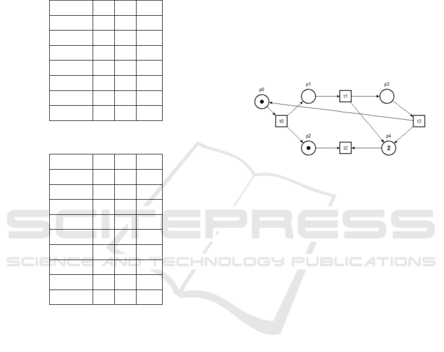
Table 1: TaskSet in ﬁrst epoch.

Epoch1 R

0 6 6

6 5 11

11 16 27

27 5 32

32 4 36

36 24 60

60 40 100

Table 2: TaskSet in second epoch.

Epoch2 R

0 6 6

6 5 11

11 16 27

27 5 32

32 4 36

36 40 76

76 8 84

84 10 94

94 6 100

These assumptions are the basis on which a model

of the scheduling algorithm can be built. We resorted

to the use of Petri Nets, that result quite intuitive in the

modeling of scheduling algorithms (Berthomieu and

Diaz, 1991; Felder et al., 1994; Leveson and Stolzy,

1987; Tsai et al., 1995). In order to represent time,

we have investigated the use of bothTimed Petri Nets

(TPN) (Ramchandani, 1974) and Coloured Petri Nets

(CPN) (Jensen, 1987). In the following part of the

article we illustrate the two kinds of models by means

of the running example, giving a comparison between

the two modeling approaches.

4 PROPOSED METHOD

A Petri Net (Petri, 1962; Murata, 1989; Peterson,

1981) is a mathematical representation of a dis-

tributed discrete system. As a modeling language, it

describes the structure of a distributed system as a bi-

partite graph with annotations. A Petri Net consists

of places, transitions and directed arcs. There may be

arcs between places and transitions but not between

places and places or transitions and transitions.

The places can hold a certain number of tokens and

the distribution of tokens on all the places of the net-

work it’s named marking. Transitions act on input

tokens according to a rule, that is named ﬁring rule.

A transition is enabled if you can ﬁre it, that is, if

there are tokens in every input place. When a tran-

sition ﬁres, it consumes tokens from its input places

and places a token in each of its output places.

Figure 1: Representation of an ordinary Petri Net.

In Figure 1 is an example of an ordinary Petri Net.

The execution of Petri Nets is not deterministic, that

is, if there are more transitions enabled at the same

time any of them can ﬁre. Since taking a transition is

not predictable in advance, Petri Nets are well suited

for modeling the concurrent behavior of distributed

systems.

Formally we can deﬁne a Petri Net as a tuple PN =

(P, T, F,W, M

) where:

• P is a ﬁnite set of places;

• T is a ﬁnite set of transition;

• F ⊆ (PxT ) ∪ (T xP) is a set of arches;

• W : F → N represents the weight of the ﬂow rela-

tion F.

• M

: P → N is the initial marking vector, which

represents the initial state of system.

• P ∩ T =

0 and P ∪ T 6=

4.1 TPN

A Timed Petri Net is a Petri Net extended with time.

In Timed Petri Nets, the transitions ﬁre in ”real-time”,

i.e., there is a (deterministic or random) ﬁring time

associated with each transition, the tokens are re-

moved from input places at the beginning of ﬁring,

and are deposited into output places when the ﬁring

terminates. Formally we can deﬁne a Timed Petri

Net (Ramchandani, 1974) as a tuple T PN = (PN, I)

where:

AMARETTO 2016 - International Workshop on domAin speciﬁc Model-based AppRoaches to vEriﬁcaTion and validaTiOn

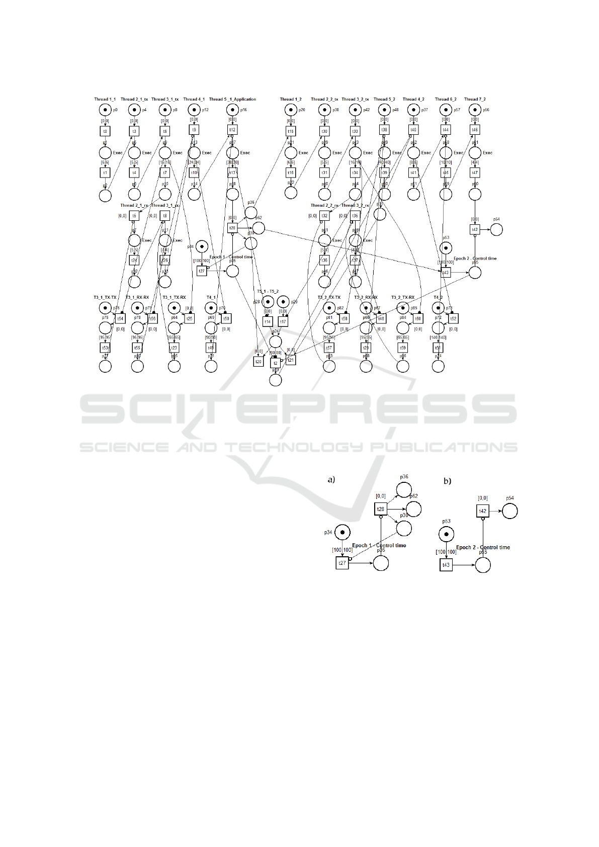
Figure 2: Timed Petri Net model for a ﬁxed scheduler.

• PN is a standard Petri Net;

• I : T → N × N is a function that maps each transi-

tion to a bounded static interval

• P ∩ T =

0 and P ∪ T 6=

In Figure 2 is reported the model generated with

the tool TINA (Berthomieu and Vernadat, 2006) for a

ﬁxed scheduler (Grolleau and Choquet-Geniet, 2002;

Barreto et al., 2004; Aalst, 1996). As we can see the

representation with TPN is a little bit chaotic and rep-

resenting larger sets of tasks could be very difﬁcult.

Looking at the model we can underline some diagram

parts which are used for the veriﬁcation of constraints

(Tsai et al., 1995):

• Check for the Total Time

The network used to control the time of each

epoch consists of two transitions and respectively

ﬁve and three places. Taking into consideration

the network a) in Figure 3, the transition t27

counts the total time available for the execution

in the epoch. When the time available ends, the

token content in place p34 is moved in place p35

and inhibits the passage of the token, from the last

thread running, in places p36, p62 and p30.

If this happens it means that the execution time in

this epoch is not the one expected. If, however,

the performance ends too soon the transition t28

will not be inhibited by p35 place and pass tokens

in places p36, p62 and p30, decreeing the passage

of the positive control and the start of the second

epoch.

Figure 3: Diagram of epoch control block.

• Check Constrains on T

The network in Figure 4 models the various con-

trols on the execution times for T

. For example

the last block checks that between the ﬁrst execu-

tion of T

in the ﬁrst epoch and the second execu-

tion in the second epoch, at least 65 milliseconds

have expired. The transition t25 is enabled when

the task is running and, if the task completes be-

fore the time set in the transition t23, scheduling

can continue. Otherwise, if the task does not com-

plete within the speciﬁed time, the inhibitor arc

Petri Nets Modeling for the Schedulability Analysis of Industrial Real Time Systems

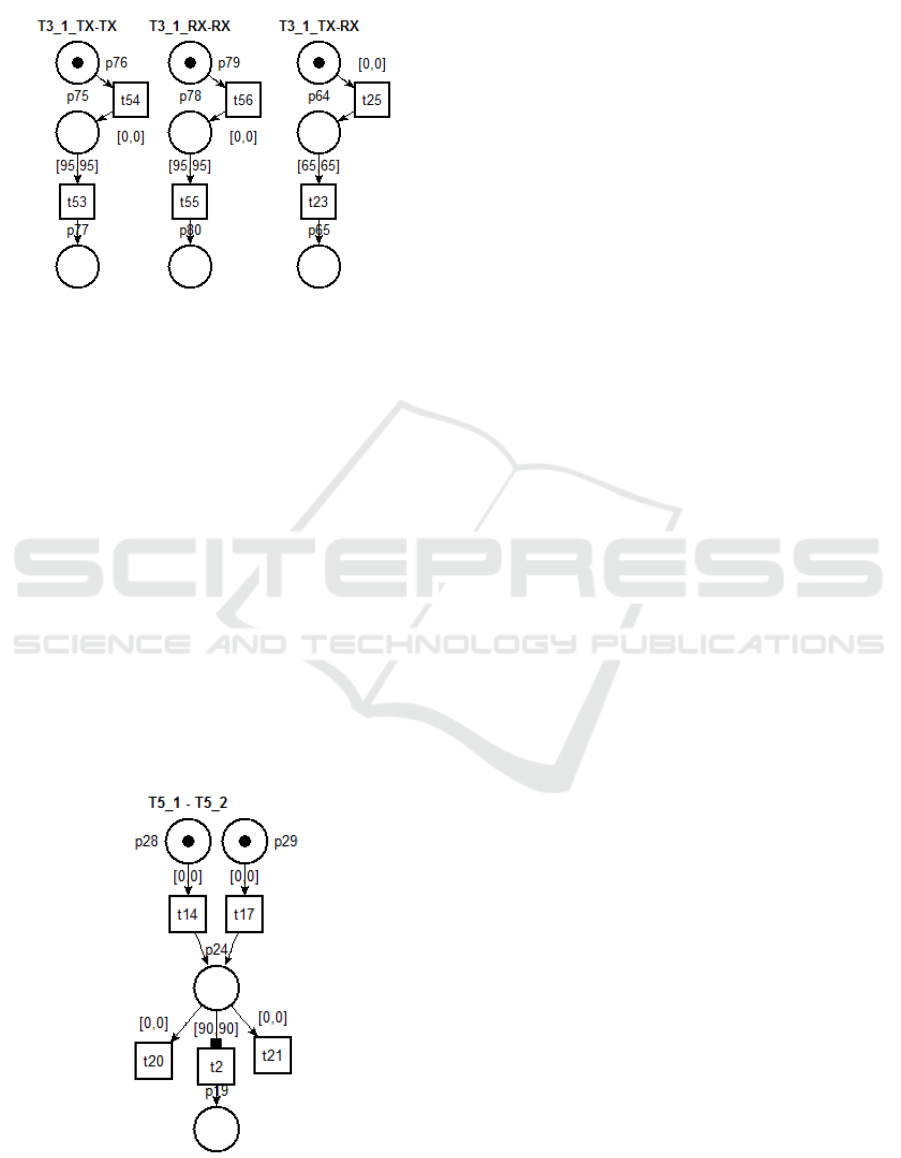
that starts from p65 does not allow the scheduler

to continue.

Figure 4: Diagram of block for the veriﬁcation of con-

straints on task T

• Checking the Scheduled Time between Two

Epochs

The network in Figure 5 monitors the execution

time of a task between the two epochs. The transi-

tions t14 and t17 are enabled when the task is run

in both the ﬁrst and the second period. This starts

the timer of transition t2. If the task completes

before the time set in the transition, the schedul-

ing can continue. Otherwise, if the task does not

complete within the speciﬁed time, the inhibitor

arc that starts from p19 does not allow the sched-

uler to continue.

With this model and TINA tool we are able to under-

stand if the hypothesized schedule is correct, and in

fact if all checks are satisﬁed we can found a token

in p54, otherwise the tool stops the simulation on the

place that generated the error.

Figure 5: Check block for the scheduled time between two

epoch for task T

4.2 CPN

An ordinary PN has no types and no modules, only

one kind of tokens and the net is ﬂat. With CPNs it is

possible, instead, to use data types and complex data

manipulation. In fact each token has attached a data

value called the token colour, which deﬁnes the range

of values that the attributes can assume and the oper-

ations applicable in the same way of a variable type

in any programming language. The types can be ba-

sic types or structured types, the latter deﬁned by the

user. The token colours can be investigated and mod-

iﬁed by the occurring transitions.

With CPNs it is possible to build a hierarchical de-

scription and for this reason a large model can be ob-

tained by combining a set of submodels.

In Figure 6 the model of the running example gener-

ated with CPN tools 4.0 (Jensen et al., 2007) is re-

ported. As we can see the representation with CPN

is more concise than the one seen with TPN, for ex-

ample in one place we can represent all the tasks of

the set. The tasks are represented as a list of objects

and each one is represented by a token that have two

attributes: a string that contains the name and one in-

teger that represent the WCET C

of the task.

The veriﬁcation of the constraints on the exe-

cution time of the thread are realized through some

functions listed on the transitions. On the ﬁrst and

second transitions named ”Put”, for example, we can

ﬁnd respectively the functions called [verifyTh3 ()]

and [verify2Th3 ()]. These two functions implement

the constraint that between the two executions of T

cannot elapse less than 65 milliseconds. The func-

tions are deﬁned as follows:

fun verifyTh3((n,t)::l) =

if n="Thread3" andalso

intTime() > 65

then false else true

fun verify2Th3(((n,t)::l)) =

if n="Thread3" andalso

(intTime()-100) > 65

then false else true

The function checks if the token in input to the

transition represents the task 3, and veriﬁes that the

current simulation time (obtained with the function

intTime()) is less than 65 units. If the constraint is not

respected, the transition is not enabled.

On the transition ”End” we can ﬁnd a function named

[verifyTime()] that checks all the other constraints

(the function is similar to the one above) except that

the one on T

that is represented by function [veri-

fyTh5ctime()] placed as guard on the same transition.

The modeling of this last constraint, speciﬁc for task

, requires to save in a variable the timing at which

AMARETTO 2016 - International Workshop on domAin speciﬁc Model-based AppRoaches to vEriﬁcaTion and validaTiOn

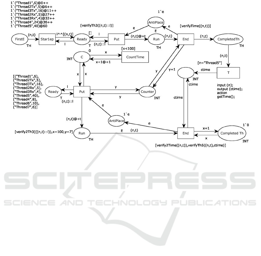
Figure 6: Coloured Petri Net model for a ﬁxed scheduler.

the token of the T

exits from the ”Run” place in the

ﬁrst epoch. This has been achieved through the tran-

sition ”T” with the pattern input, output, action where

we take a variable in input (variable n) and by the ac-

tion (getTime() function) we generate an output (vari-

able ctime). This transition is enabled only for T

we can see from the guard on the arch. So the variable

that we have obtained could be used in the function:

fun verifyTh5 ((n, t), ctime)=

if n= "Thread5" andalso

(intTime () - ctime) >= 90

{then false else true}

Similarly to the modeling done with TPN, also the

simulation of the CPN model by means of the CPN

Tools 4.0 stops if one of the constraint is not satisﬁed,

so the user is able to understand where the problem is

located.

4.3 Comparison between TPN and CPN

The experiments have allowed a comparison between

the two Petri Nets dialects, in particular enlightening

the following points:

The TPN model is difﬁcult to read, and the addition

of further tasks would result in a huge increase of the

places and transitions number, making it more and

more unreadable. This increase is due to the fact that:

• Any place can hold a single token and the execu-

tion of a thread must be reproduced a number of

times equal to the number of modeled processes;

indeed in TPNs it is not possible to express an at-

tribute that differentiates the identity of a token.

• Time management for each thread is left to time

constraints on the transitions themselves.

• It is not possible to create aggregate objects: a

FIFO queue, for example, can be realized only

through checks by inhibitors arcs with a num-

ber of places that depends on how many threads

should be modeled (the number of places to repre-

sent the queue is equal to n

where n is the number

of threads).

The CPNs instead can represent a queue using a single

place that contains a token of type list. Time manage-

ment is left to the token using an integer and a times-

tamp. This allows to represent a large number of tasks

by simply adding tokens to the initial marking, leav-

ing the structure of the model unaffected.

The time constraints can be grouped in auxiliary func-

tions, thus simplifying size and readability of the

model. In TPNs, instead, for each thread it is nec-

essary to model a constraint through places and tran-

sitions.

With TINA and TPNs the control of time during sim-

ulation allows to easily understand the global state of

the system. The time is increased at any time unit

time. In CPNTools and CPNs if there are no transi-

tions enabled at the current time, the simulated time

count is increased in one step up to the time at which

Petri Nets Modeling for the Schedulability Analysis of Industrial Real Time Systems

at least one transition is activated.

CPNs have however resulted to be more advantageous

in terms of time spent in model design or in changes,

mainly for two reasons:

1. constraints can be simply modeled by a guard on

the transition, expressed by a function written in

pseudo code, which is easier to express;

2. to populate the model with new tasks it is not nec-

essary to draw new graphic elements but just add

an entry to the related place;

We have experienced that the time spent in CPN mod-

eling is at the end more than half that spent in TPN

modeling.

5 CONCLUSIONS

We have applied the two modeling options sketched

above to different scheduling algorithms and differ-

ent sets of tasks as well. The quite straightforward

conclusion is that the CPN modeling is more advan-

tageous in terms of size and readability of the model,

and in terms of adaptability of the model to different

task sets.

It is indeed easier with CPN to instantiate the same

model, for the same scheduling algorithms, on a dif-

ferent set of tasks, and this is what is important in the

daily application of this modeling framework. Since

essentially only the characteristics of the taskset need

to be changed for a new, or modiﬁed, speciﬁc appli-

cation, the overall time to analyse a new taskset, sum-

ming up the time to produce a model of the sched-

ule of a new speciﬁc application, to run a simulation

and to analyse the simulation is about two hours with

a TPN modeling and about one hour with the CPN

modeling. Anyway, this time compares with the much

longer time (eight hours) needed by the empirical ap-

proach previously used, and therefore is convenient in

both cases.

Even if some rework is needed due to a negative re-

sponse of the simulation, the information returned by

the simulation helps understanding where the prob-

lem lies, indicating the solution to the problem. Usu-

ally one rework cycle is at most needed, so the overall

cost is anyway reduced.

For this reason we have not considered convenient

to investigate solutions based on counterexample gen-

erated by a model checker (Guillaume Gardey, 2005),

able to provide automatically the taskset parameters

satisfying the scheduling requirements.

The low cost of the simulation based solution has

an obvious positive impact on the costs of the process

of instantiating a generic application to a new speciﬁc

application for marketing a new product or variant.

This process is currently under experimentation in our

partner company, with the aim of introducing it in the

routine customization process. An help for this intro-

duction could come from providing tools to support

an easier instantiation of the generic models into spe-

ciﬁc ones, so that the use of CPN is transparent to the

ﬁnal user who only sees the simulation results. This

objective requires also a facility to explain the reasons

of a negative response without showing the underly-

ing CPN model. This is considered as future work.

ACKNOWLEDGEMENTS

We wish to thank Marco Bartolozzi, Daniele

Marchetti and Luca Santi for their contribution to the

conducted modeling experiments.

REFERENCES

van der Aalst, W. M. P. (1996). Petri Net based schedul-

ing. In Operations-Research-Spektrum vol.18 (219-

229). Springer-Verlag.

Alur, Rajeev and Dill, David (1992). The theory of timed

automata. In 17th Real-Time: Theory in Practice,

Lecture Notes in Computer Science vol.600 (45-73).

Springer.

Barreto, R., Cavalcante, S., and Maciel, P. (2004). A

time Petri Net approach for ﬁnding preruntime sched-

ules in embedded hard real-time systems. In Dis-

tributed Computing Systems Workshops (846-851),

2004. Proceedings. IEEE.

Berthomieu, B. and Vernadat, F. (2006). Time Petri Nets

analysis with TINA. In Quantitative Evaluation of

Systems (123-124), 2006. IEEE.

Berthomieu, B., Diaz, M. (1991) Modeling and Veriﬁca-

tion of Time dependent system using Time Petri Nets.

IEEE Transactions on Software Engineering, vol. 17 ,

no. 3 (259-273). IEEE.

Buttazzo, G. (2011). Hard Real-Time Computing System.

Springer, New York, 3rd edition.

Cenelec (1996). Cenelec en 50128. In Railway Appli-

cations - Communications, Signalling and Processing

Systems - Software for Railway Control and Protec-

tion Systems.

CPNTools (2015). <http://http://cpntools.org/>.

Fantechi, A. (2013) Twenty-Five Years of Formal Meth-

ods and Railways: What Next? SEFM Workshops

2013, Lecture Notes in Computer Science vol.8368

(167-183), Springer.

Felder, M., Mandrioli, D., Morzenti, A. (1994) Prov-

ing Properties of Real-Time Systems through Logical

Speciﬁcations and Petri Net Models, IEEE Transac-

tions on Software Engineering, vol.20, no.2 (127-141)

AMARETTO 2016 - International Workshop on domAin speciﬁc Model-based AppRoaches to vEriﬁcaTion and validaTiOn

Grolleau, E., Choquet-Geniet, A. (2002). Off-line compu-

tation of real-time schedules using Petri Nets. In Dis-

crete Event Dynamic Systems, vol.12, no.3 (311-333).

Springer.

Guillaume Gardey, Didier Lime, Morgan Magnin, and

Olivier (H.) Roux (2005). Romo: A tool for analyzing

time Petri nets. In 17th International Conference on

Computer Aided Veriﬁcation (CAV05), Lecture Notes

in Computer Science vol.3576 (418-423), Edinburgh,

Scotland. Springer.

Jensen, K. (1987). Coloured Petri Nets. In Petri Nets:

Central Models and Their Properties. Lecture Notes

in Computer Science, vol.254 (248-299), Springer.

Jensen, K., Kristensen, L. M., and Wells, L. (2007).

Coloured Petri Nets and CPN tools for modelling and

validation of concurrent systems. In International

Journal on Software Tools for Technology Transfer,

vol.9, no.3 (213-254) Springer-Verlag.

Leveson, N. G., Stolzy, J. L. (1987) Safety Analysis using

Petri Nets. IEEE Transactions on Software Engineer-

ing, vol.13, no.3

Liu, C. L. and Layland, J. W. (1973). Scheduling algo-

rithms for multiprogramming in a hard-real-time envi-

ronment. In Journal of the ACM, vol.20, no.1 (46-61).

ACM.

Murata, T. (1989). Petri Nets: Properties, analysis and ap-

plications. In Proceedings of the IEEE, vol.77, no.4

(541-580). IEEE.

Peterson, J. L. (1981). Petri Net Theory and the Modeling

of Systems. Prentice Hall PTR, Upper Saddle River,

NJ, USA.

Petri, C. A. (1962). Kommunikation mit automaten. In PhD

thesis. Universitat Hamburg.

Ramchandani, C. (1974). Analysis of asynchronous con-

current systems by Timed Petri Nets. Massachusetts

Institute of Technology.

Stankovic, J. (1988). Misconceptions About Real-Time

Computing. IEEE Computer, vol.21 (10-19). IEEE.

TINA (2015). <http://http://http://projects.laas.fr/tina//>.

Tsai, J., Jennhwa Yang, S., and Chang, Y.-H. (1995).

Timing constraint Petri Nets and their application to

schedulability analysis of real-time system speciﬁca-

tions. In IEEE Transactions on Software Engineering,

vol. 21, no. 1 (32-49). IEEE.

Petri Nets Modeling for the Schedulability Analysis of Industrial Real Time Systems