
Document-oriented Models for Data Warehouses
NoSQL Document-oriented for Data Warehouses
Max Chevalier
1
, Mohammed El Malki
1,2
, Arlind Kopliku
1
, Olivier Teste
1
and Ronan Tournier
1
1
Université de Toulouse, IRIT (UMR 5505), Toulouse, France
2
Capgemini, Toulouse, France
Keywords: NoSQL, Document-oriented, Data Warehouse, Multidimensional Data Model, Star Schema.
Abstract: There is an increasing interest in NoSQL (Not Only SQL) systems developed in the area of Big Data as
candidates for implementing multidimensional data warehouses due to the capabilities of data
structuration/storage they offer. In this paper, we study implementation and modeling issues for data
warehousing with document-oriented systems, a class of NoSQL systems. We study four different mappings
of the multidimensional conceptual model to document data models. We focus on formalization and cross-
model comparison. Experiments go through important features of data warehouses including data loading,
OLAP cuboid computation and querying. Document-oriented systems are also compared to relational
systems.
1 INTRODUCTION
In the area of Big Data, NoSQL systems have
attracted interest as mean for implementing
multidimensional data warehouses (Chevalier et al,
2015a), (Chevalier et al, 2015b), (Mior, 2014), (Dede
et al, 2013), (Schindler, 2012). The proposed
approaches mainly rely on two specific classes of
NoSQL systems, namely document-oriented systems
(Chevalier et al, 2015a) and column oriented systems
(Chevalier et al, 2015b), (Dede et al, 2013). In this
paper, we study further document-oriented systems in
the context of data warehousing.
In contrast to Relational Database Management
Systems (RDBMS), document-oriented systems,and
many other NoSQL systems, are famous for
horizontal scaling, elasticity, data availability, and
schema flexibility. They can accommodate
heterogeneous data (not all conforming to one data
model); they provide richer structures (arrays,
nesting…) and they offer different options for data
processing including map-reduce and aggregation
pipelines. In these settings, it becomes interesting to
investigate for new opportunities for data
warehousing. On one hand, we can exploit scalability
and flexibility for large-scale deployment. On the
other hand, we can accommodate heterogeneous data
and consider mapping to new data models. In this
setting, document-oriented systems become natural
candidates for implementing data warehouses.
In this paper, we consider four possible mappings
of the multidimensional conceptual model into
document logical models. This includes simple
models that are analogous to relational database
models using normalization and denormalization. We
also consider models that use specific features of the
document-oriented system such as nesting and
schema flexibility. We instantiate a data warehouse
using each of the models and we compare each
instantiation with each other on different axes
including: data loading, querying, and OLAP cuboid
computation.
2 RELATED WORK
Multidimensional databases are mostly implemented
using RDBMS technologies (Chaudhuri et al, 1997),
(Kimball, 2013). Considerable research has focused
on the translation of data warehousing concepts into
relational logical level (Bosworth et al, 1995),
(Colliat et al, 1996), (called R-OLAP). Mapping rules
are used to convert structures of the conceptual level
(facts, dimensions and hierarchies) into a logical
model based on relations (Ravat, et al, 2006).
142
Chevalier, M., Malki, M., Kopliku, A., Teste, O. and Tournier, R.
Document-oriented Models for Data Warehouses - NoSQL Document-oriented for Data Warehouses.
In Proceedings of the 18th International Conference on Enterprise Information Systems (ICEIS 2016) - Volume 1, pages 142-149
ISBN: 978-989-758-187-8
Copyright
c
2016 by SCITEPRESS – Science and Technology Publications, Lda. All rights reserved

There is an increasing attention towards the
implementation of data warehouses with NoSQL
systems (Chevalier et al, 2015a), (Zhao et al, 2014),
(Dehdouh et al, 2014), (Cuzzocrea et al, 2013). In
(Zhao et al, 2014), the authors implement a data
warehouse into a column-oriented store (HBase). They
show how to instantiate efficiently OLAP cuboids with
MapReduce-like functions. In (Floratou et al, 2012),
the authors compare a column-oriented system (Hive
on Hadoop) with a distributed version of a relational
system (SQL server PDW) on OLAP queries.
Document-oriented systems offer particular data
structures such as nested sub-documents and arrays.
These features are also met in object-oriented and
XML like systems. However, none of the above has
met success as RDBMS for implementing data
warehouses and in particular for implementing OLAP
cuboids as we do is this paper. In (Kanade et al, 2014),
different document logical models are compared to
each other: data denormalization, normalized data;
and models that use nesting. However, this study is in
a “non-OLAP” setting.
In our previous work (Chevalier et al, 2015a),
(Chevalier et al, 2015b) we have studied 3 column-
oriented models and 3-document-oriented models for
multidimensional data warehouses. We have focused
on direct translation of the multidimensional model to
NoSQL logical models. However, we have
considered simple models (models with few
document-oriented specific features) and the
experiments were at an early stage. In this paper, we
focus on more powerful models and our experiments
cover most of data warehouse issues.
3 DOCUMENT DATA MODEL
FOR DATA WAREHOUSES
We distinguish three abstraction levels: conceptual
model (Golfarelli et al, 1998), (Annoni, et al, 2006)
that is independent of technologies, logical model that
corresponds to one specific technology but software
independent, physical model that corresponds to one
specific software. The multidimensional schema is
the reference conceptual model for data warehousing.
We will map this model to document-oriented data
models.
3.1 Multidimensional Conceptual
Model
Definition 1. A multidimensional schema, namely E,
is defined by (F
E
, D
E
, Star
E
) where: F
E
= {F
1
,…, F
n
}
is a finite set of facts, D
E
= {D
1
,…, D
m
} is a finite set
of dimensions, and Star
E
: F
E
→ 2
is a function that
associates facts of F
E
to sets of dimensions along
which it can be analyzed (2
is the power set of D
E
).
Definition 2. A dimension, denoted D
i
∈D
E
(abusively noted as D), is defined by (N
D
, A
D
, H
D
)
where: N
D
is the name of the dimension;
=
{
,…,
}
U{
,…,
}
is a set of dimension
attributes; and
={
,…
} is a set of
hierarchies. A hierarchy can be as simple as the
example {“day, month, year”}.
Definition 3. A fact, F∈F
E
, is defined by (N
F
, M
F
)
where: N
F
is the name of the fact, and
=
{
,…,
} is a set of measures. Typically, we apply
aggregation functions on measures. A combination of
dimensions represents the analysis axis, while the
measures and their aggregations represent the
analysis values.
3.2 Document-oriented Logical Model
Here, we provide key definitions and notation we will
use to formalize documents. Documents are grouped
in collections. We refer to such a document as C(id).
Definition 4. A document corresponds to a set of
key-values. A unique key identifies every document;
we call it identifier. Keys define the structure of the
document; they act as meta-data. Each value can be
an atomic value (number, string, date…) or a sub-
document or array. Documents within documents are
called sub-documents or nested documents.
Definition 5. The document structure/schema
corresponds to a generic document without atomic
values i.e. only keys.
We use the colon symbol “:” to separate keys
from values, “[]” to denote arrays, “{}” to denote
documents and a comma “,” to separate key-value
pairs from each other.
With the above notation, we can provide an
example of a document instance. It belongs to the
“Persons” collection, it has 30001 as identifier and it
contains keys such as “name”, “addresses”, “phone”.
The addresses value corresponds to an array and the
phone value corresponds to a sub-document.
Persons(30001):
{name:“John Smith”,
addresses:
[{city:“London”, country:“UK”},
{city:“Paris”, country:“France”}],
phone:
{prefix:“0033”, number:“61234567”}}
The above document has a document schema:
{name, addresses: [{city, country}],
phone: {prefix, number}}
Document-oriented Models for Data Warehouses - NoSQL Document-oriented for Data Warehouses
143

Another way to represent a document is through
all the paths within the document that reach the
atomic values. A path p of a document instance with
identifier
id is described as p=C(id):k
1
:k
2
:…k
n
:a
where
k
1
, k
2
,… k
n
:a are keys within the same path
ending at an atomic value
a.
In a same collection it is possible to have
documents with different structures: the schema is
specific at the document level. We define the
collection model as the union of all schemas of all
documents. A collection C that accepts two sub-
models S
1
and S
2
, can be written as S
C
={S
1
, S
2
}. This
formalism will be enough for our purposes.
3.3 Document-oriented Models for
Data Warehousing
In this section, we present document models that we
will use to map the multidimensional data model. We
refer here to the multidimensional conceptual model as
described in section 3 and we describe and illustrate
four logical data models. Each time we describe the
model for a fact F (with name N
F
) and its dimensions
D∈Star
E
(F)
(each dimension has a name N
D
).
We will illustrate each model with a simple
example. We consider the fact “LineOrder” and only
one dimension “Customer”. For “LineOrder”, we
have three measures “l_quantity”, “l_shipmode” and
“l_price”. For “Customer”, we have three attributes
“c_name”, “c_city” and “c_nation_name”.
The chosen models are diverse each one with
strengths and weaknesses. They are also useful to
illustrate the modeling issues in document-oriented
systems. Models M0 and M2 are equivalent to data
denormalization and normalization in RDBMS.
Model M1 is similar to M0, but it adds some more
structure (meta-data) to documents. This model is
interesting to see if extra meta data is penalizing (in
terms of memory usage, query execution, etc.). Model
M3 is similar to M2, but everything is stored in one
collection. M3 exploits schema flexibility i.e. it stores
in one collection documents of different schema.
Each model is defined, formalized and illustrated
below:
Model M0, Flat: It corresponds to a denormalized
flat model. Every fact from F is stored in a collection
C
F
with all attributes of its dimensions Star
E
(F). It
corresponds to denormalized data (in RDBMS).
Documents are flat (no nesting), all attributes are at
the same level. The schema S
F
of the collection C
F
is:
={id,
,
,…
,
,
,…
,
,
…
,…}
e.g.
{id:1,
l_quantity:4,
l_shipmode:“mail”,
l_price:400.0,
c_name:“John”,
c_city:“Rome”,
c_nation_name:“Italy”}
Model M1, Deco: It corresponds to a denormalized
model with more structure (meta-data). It is similar to
M0, because every fact F is stored in a collection C
F
with all attributes of its dimensions Star
E
(F). In each
document, we group measures together in a sub-
document with key N
F
. Attributes of one dimension
are also grouped together in a sub-document with key
N
D
. This model is simple, but it illustrates the
existence of non-flat documents. The schema S
F
of
the C
F
is:
=
,N
:
,
,..
,
:{
,
,…
,
:{
,
,…
},…}
e.g.
{id:1,
LineOrder:
{l_quantity:4,
l_shipmode:“mail”,
l_price:400.0},
Customer:
{c_name:“John”,
c_city:“Rome”,
c_nation_name:“Italy”}}
Model M2, Shattered: It corresponds to a data model
where fact records are stored separately from
dimension records to avoid redundancy, equivalent to
normalization. The fact F is stored in a collection C
F
and each dimension D∈Star
E
(F) is stored in a
collection C
D
. The fact documents contain foreign
keys towards the dimension collections. The schema
S
F
of C
F
and the schema
of a dimension collection
C
D
are as follows:
={
,
,
,…
,
,
,…}
={
,
,
,…
}
e.g.
{id:1,
l_quantity:4,
l_shipmode:“mail”,
l_price:400.0,
c_id:4} ∈C
{id:4,
c_name:“John”,
c_city:“Rome”,
c_nation_name:“Italy”} ∈C
ICEIS 2016 - 18th International Conference on Enterprise Information Systems
144

Model M3, Hybrid: It corresponds to a hybrid model
where we store documents of different schema in one
collection. We store everything in one collection, say
C
F
. We store the fact entries with a schema S
F
.
Dimensions are stored within the same collection, but
each with its complete schema S
D
.
We need to keep references from fact entries
towards the corresponding dimension entries. This
model is similar to M2, at the difference of storing
everything in one collection.
This model is interesting, because if we use
indexes properly, we can access quickly the
dimension attributes and all corresponding facts e.g.
with an index on c_custkey, we access quickly all
sales of a given customer.
The schemas S
F
and S
D
are:
={,
,
,…
,
,
,…} ;
={
,
,
,…
}
e.g.
{id:1,
l_quantity:4,
l_shipmode:“mail”,
l_extended_price:400.0,
c_custkey:2,
c_datekey:3} ∈C
{id:2,
custkey: 4,
c_name: “John”,
c_city: “Rome”,
c_nation_name:“Italy”,
c_region_name:“Europe”} ∈C
{id:3,
date_key:1,
d_date:10,
d_month:“January”,
d_year:2014} ∈C
In Table 1, we summarize the mapping of the
multidimensional model to our logical models. For
every dimension attribute or fact measure, we show
the corresponding collection and path within a
document structure.
Table 1: Mapping of the multidimensional schema to the
logical data models.
∀
D
∈
D
O
∀
a
∈
A
D
∀
m
∈
M
F
collection path collection path
M0
C
F
a C
F
m
M1
C
F
N
D
:a C
F
N
F
:m
M2
C
D
a C
F
m
M3
C
F
a C
F
m
4 EXPERIMENTS
4.1 Experimental Setup
The experimental setup is briefly introduced and then
detailed in the next paragraphs. We generate 4
datasets according to the SSB+, Star schema
benchmark (Chevalier et al, 2015c), (Oneil et al,
2009), which is itself a derived from the TPC-H
benchmark. TPC-H is a reference benchmark for
decision support systems. The benchmark is extended
to generate data compatible to our document models
(M0, M1, M2, M3). Data is loaded in MongoDB v2.6,
a popular document-oriented system. On each
dataset, we issue sets of OLAP queries and we
compute OLAP cuboids on different combinations of
dimensions. Experiments are done in single-node and
a distributed 3-nodes cluster setting.
For comparative reasons, we also load two
datasets in PostgresSQL v8.4, a popular RDBMS. In
this case, dataset data corresponds to a flat model
(M0) and a star-like normalized model (M2), that we
name respectively R0 and R2. Experiments in
PostgreSQL are done in a singlenode setting.
Data. We generate data using an extended version
of the Start Schema Benchmark denoted SSB+
(Chevalier et al, 2015c), (Oneil et al, 2009). The
benchmark models a simple product retail reality. The
SSB+ benchmark models a simple product retail
reality. It contains one fact “LineOrder” and 4
dimensions “Customer”, “Supplier”, “Part” and
“Date”.
We generate data using an extended version of the
Start Schema Benchmark SSB (Oneil et al, 2009)
because it is the only data warehousing benchmark that
has been adapted to NoSQL systems. The extended
version is part of our previous work (Blind3). It makes
possible to generates raw data directly as JSON which
is the preferable data format for data loading in
MongoDB. We use improve scaling factor issues that
have been reported. In our experiments we use
different scale factors (sf) such as sf=1, sf=10 and
sf=25 in our experiments. In the extended version, the
scale factor sf=1 corresponds to approximately 10
7
records for the LineOrder fact, for sf=10 we have
approximately 10x10
7
records and so on.
Settings/Hardware/Software. The experiments
have been done in two different settings: single-node
architecture and a cluster of 3 physical nodes. Each
node is a Unix machine (CentOs) with 4 core-i5 CPU,
8GB RAM, 2TB disks, 1Gb/s network. The cluster is
composed of 3 nodes, each being a worker node and
one node acts also as dispatcher. Each node has a
MongoDB v.3.0 running. In MongoDB terminology,
Document-oriented Models for Data Warehouses - NoSQL Document-oriented for Data Warehouses
145
this setup corresponds to 3 shards (one per machine).
One machine also acts as configuration server and
client.
4.2 Document-oriented Data
Warehouses by Model
Data Loading. We report first the observations on
data loading. Data with model M0 and M1 occupy
about 4 times less space than data with models M2
and M3. For instance, at scale factor sf=1 (10
7
line
order records) we need about 4.2GB for storing
models M2 and M3, while we need about 15GB for
models M0 and M1. The above observations are
explained by the fact that data in M2 or M3 has less
redundancy. In M2 and M3 dimension data is
repeated just once.
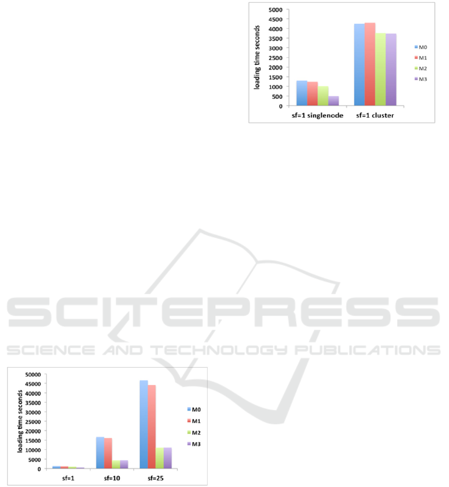
Figure 1 shows data loading times by model and
scale factor (sf=1, sf=10, sf=25) on a singlenode
setting. Loading times are as expected higher for the
data models that require more memory (M0 and M1).
In Figure 2, we compare loading times for sf=1 on
singlenode setting with the distributed setting. We
observe data loading is significantly slower in a
distributed setting than on a single machine. For
instance, model M0 data (sf=1) loads for 1306s on a
single cluster, while it needs 4246s in a distributed
setting. This is mainly due to penalization related to
network data transfer. Indeed, MongoDB balances
data load i.e. it tries to distribute equally data across
all shards implying more network communication.
Figure 1: Loading times by data models.
Querying. We test each instantiation (on 4 data
models) on 3 sets of OLAP queries (QS1, QS2, QS3).
To do so, we use the SSB benchmark query generator
that generates 3 query variants per set. The query
complexity increases from QS1 to QS3. QS1 queries
filter on one dimension and aggregate all data; QS2
queries filter data on 2 dimensions and group data on
one dimension; and QS3 queries filter data on 3
dimensions and group data on 2 dimensions.
Figure 2: Loading time comparisons on single node and
cluster.
In Table 3 and 4, we show query execution times
on all query variants with scale factor sf=1, all
models, in two settings (single node and cluster). For
the queries with 3 variants, results are averaged
(arithmetic mean). In Table 3, we can compare
averaged execution times per query and model in the
single node setting. In Table 4, we can compare
execution times in the distributed (cluster) setting.
We observe that for some queries some models
work better and for others some other models work
better. We would have expected queries to run faster
on models M0 and M1 because data is in a
denormalized fashion (no joins needed). This is
surprisingly not the case. Query execution times are
comparable across all models and sometimes queries
run faster for models M2 and M3. This is partly
because we could optimize queries choosing from the
MongoDB rich palette: aggregation pipeline,
map/reduce, simple queries and procedures. For M2
and M3, we need to join data from more than one
document at a time. When we do not write the most
efficient MongoDB query and/or when we join all
data needed for the query before any filtering,
execution times can be significantly higher. Instead
we apply filters before joins and then we use the
aggregation pipeline , map/reduce functions, simple
queries or procedures. We also observed the SSB
queries had high selectivity. We could filter most
records before needing any join. To test selectivity
impact, we tested querying performance on another
query Q4 that is obtained by modifying one of the
queries from QS1 to be more selective. On this new
query set we have about 500000 facts after filtering.
We observe that query execution on data with models
M0 and M1 is lower about 20-30%. Meanwhile, on
data with models M2 and M3 query execution is
respectively about 5-15 times slower. This is purely
due to the impact of joins that are not supported by
document-oriented systems in general.
ICEIS 2016 - 18th International Conference on Enterprise Information Systems
146
To fully understand the impact of joins on data
with models M2 and M3, we conducted another
experiment when we join all data i.e. we basically
generate data with model M0 starting from data with
model M2 and M3. In the most performant
approaches we could produce, we observed 1010
minutes for M2 and 632 minutes for M3 on sf=1. This
is a huge delay. We can conclude that data joins can
be a major limitation for document-oriented system.
When joins are poorly supported, data models such as
M2 and M3 are not interesting.
In Table 3 and Table 4, we can also compare
query execution times in singlenode setting with
respect to distributed setting. We observe that query
execution times are generally better in a distributed
setting. For many queries, execution times improve 2
to 3 times depending on the cases. In a distributed
setting, query execution is penalized by network data
transfer, but it is improved by parallel computation.
When queries are executed on data with models M2
and M3, improvement on the distributed setting is less
important (less than 1.5 times).
4.3 OLAP Cuboids with Documents
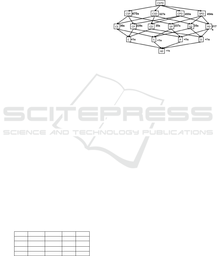
OLAP Cuboid. It is common in OLAP applications
to pre-compute analysis cuboids that aggregate fact
measures on different dimension combinations. In our
example (SSB dataset), there are 4 dimensions C:
Customer, S: Supplier, D: Date and P: Part. In Figure
3, we show all possible dimension combinations.
Data can be analyzed on no dimension (all), 1
dimension, 2 dimensions or 3 dimensions or 4
dimensions. Cuboid names are given with dimension
initials, e.g. CSP stands for cuboid on Customer,
Supplier and Part. In Figure 3, we show for
illustration purposes the computation time for a
complete lattice in M0. In this case, we compute
lower level cuboids from the cuboid just on top to
make things faster.
In Table 2 we show the average time needed to
compute an OLAP cuboid of x dimensions (x can be
3, 2, 1, 0, i.e. group on 3 dimensions, 2 dimensions
and so on). Cuboids are produced starting from data
on any of the models M0, M1, M2, or M3.
Table 2: Average aggregation time per lattice level on
single node setting.
M0 M1 M2 M3
3D 423s 460s 303s 308s
2D 271s 292s 157s 244s
1D 196s 201s 37s 44s
all 185s 191s 37s 27s
We observe that we need less time to compute the
OLAP cuboid with M2 and M3. This is because we
do not denormalize data, i.e. we group only on foreign
keys. If we need cuboids that use other dimension
attributes, the computation time is significantly
higher.
Figure 3: Computation time for each OLAP cuboid with M0
on single node (letters are dimension names: C=Customer,
S=Supplier, D=Date, P=Part).
4.4 Document-oriented Data
Warehouses versus Relational
Data Warehouses
In this section, we compare loading times and
querying between data warehouse instantiations on
document-oriented and relational databases. In
document-oriented systems, we consider the data
model M0, because it performs better than the others.
In the relational database, we consider two models R0
and R2 mentioned earlier. For R0, data is
denormalized, everything is stored in one table: fact
and dimension data. For R2, data is stored in a star-
like schema i.e. the fact data is stored in one table and
each dimension data is stored in a separate table.
Loading. First of all, we observe that relational
databases demand for much less memory than
document-oriented systems. Precisely, for scale
factor sf=1, we need 15GB for data model M0 in
MongoDB. Instead we need respectively 4.2GB and
1.2GB for data models R0 and R2 in PostgreSQL.
This is easily explained. Document-oriented systems
repeat field names on every document and
specifically in MongoDB data types are also stored.
To store data with flat models we need about 4 times
more space, due to data redundancy. The same
proportions are also observed on loading times.
Querying. We first compare query performance
on the 4 query sets defined earlier (QS1, QS2, QS3,
Q4) on a single node. We observe immmediately that
queries run significantly faster on PostgreSQL (20 to
100 times). This is partly due to the relatively high
Document-oriented Models for Data Warehouses - NoSQL Document-oriented for Data Warehouses
147
selectivity of the considered queries. Almost all data
fits in memory.
Table 3: Query execution time per model, single node
setting.
sf=1 M0 M1 M2 M3
Q1.1 62s 62s 37s 94s
Q1.2 59s 61s 33s 91s
Q1.3 58s 58s 33s 86s
Q1 avg 60s 61s 34s
✓
90s
Q2.1 36s 39s 85s 105s
Q2.2 37s 41s 83s 109s
Q2.3 37s 40s 83s 109s
Q2 avg 37s
✓
40s 84s 108s
Q3.1 36s 36s 89s 100s
Q3.2 40s 40s 89s 104s
Q3.3 38s 38s 92s 104s
Q3 avg 38s
✓
38s 90s 103s
Q4 74s
✓
77s 689s 701s
Table 4: Query execution time per model, cluster setting.
sf=1 M0 M1 M2 M3
Q1.1
Q1.2
Q1.3
150s
141s
141s
152s
142s
141s
50s
47s
47s
129s
125s
127s
Q1 avg 144s 145s 48s
✓
127s
Q2.1
Q2.2
Q2.3
140s
140s
140s
140s
142s
138s
85s
84s
86s
107s
103s
111s
Q2 avg 140s 145s 85s
✓
107s
Q3.1
Q3.2
Q3.3
137s
140s
142s
138s
143s
143s
97s
99s
98s
105s
107s
108s
Q3 avg 139s 141s 98s 106s
Q4 173s
✓
180s 747s 637s
In addition, we considered OLAP queries that
correspond to the computation of OLAP cuboids.
These queries are computationally more expensive
than the queries considered previously (QS1, QS2,
QS3, Q4). More precisely, we consider here the
generation of OLAP cuboids on combinations of 3
dimensions. We call this query set QS5.
Average execution times on all query sets are
shown in Table 5. We observe that the situation is
reversed on this query set. Query execution times are
comparable to each other. Queries run faster on
MongoDB with data model R0 (singlenode) than on
PostgresSQL. Queries run fastest on PostgreSQL
with data model R2. MongoDB is faster if we
consider the distributed setting.
Table 5: Average querying times by query set and approach.
single node sf=1 M0 R0 R2
QS1 144s 7s 1s
QS2 140s 3s 2s
QS3 139s 3s 2s
Q4 173s 3s 1s
QS5 423s 549s 247s
On these queries we have to keep in memory
much more data than for queries in QS1, QS2, QS3
and QS4. Indeed, on the query sets QS1, QS2, QS3
and QS4 the amount of data to be processed is
reduced by filters (equivalent of SQL where
instructions). Then data is grouped on fewer
dimensions (0 to 2). The result is fewer data to be kept
in memory and fewer output records. Instead for
computing 3 dimensional cuboids, we have to process
all data and the output has more records. Data will not
fit in main memory in MongoDB or PostgreSQL.
Nonetheless MongoDB seems suffering less this
aspect than PostgreSQL.
We can conclude that MongoDB scales better
when the amount of data to be processed increases
significantly. It can also take advantage of
distribution. Instead, PostgresSQL performs very
well when all data fits in main memory.
5 CONCLUSIONS
In this paper, we have studied the instantiation of data
warehouses with document-oriented systems. For this
purpose, we formalized and analyzed four logical
models. Our study shows weaknesses and strengths
across the models. We also compare the best
performing data warehouse instantiation in
document-oriented systems with 2 instantiations in
relational database.
Depending on queries and data warehouse usage,
we observe that the ideal model differs. Some models
require less disk space, more precisely M2 and M3.
This is due to the redundancy of data in models M0
and M1 that is avoided with models M2 and M3. For
highly selective queries, we observe no ideal model.
Queries run sometimes faster on one model and
sometimes on another. The situation changes fast
when queries are less selective. On data with models
M2 and M3, we observe that querying suffers from
joins. For queries that are poorly selective, we
observe a significant impact on query execution times
making these models non-recommendable.
We also compare instantiations of data
warehouses on a document-oriented system with a
relational system. Results show that RDBMS is faster
on querying raw data. But performance slows down
quickly when data does not fit on main memory.
Instead, the analysed document-oriented system is
shown more robust i.e. it does not have significant
performance drop-off with scale increase. As well, it
is shown to benefit from distribution. This is a clear
advantage with respect to RDBMS that do not scale
ICEIS 2016 - 18th International Conference on Enterprise Information Systems
148

well horizontally; they have a lower maximum
database size than NoSQL systems.
In the near future, we are currently studying
another document-oriented system and some column-
oriented systems with the same objective.
ACKNOWLEDGEMENTS
This work is supported by the ANRT funding under
CIFRE-Capgemini partnership.
REFERENCES
E. Annoni, F. Ravat, O. Teste, and G. Zurfluh. Towards
Multidimensional Requirement Design. 8th
International Conference on Data Warehousing and
Knowledge Discovery (DaWaK 2006), LNCS 4081,
p.75-84, Krakow, Poland, September 4-8, 2006.
A. Bosworth, J. Gray, A. Layman, and H. Pirahesh. Data
cube: A relational aggregation operator generalizing
group-by, cross-tab, and sub-totals. Tech. Rep.
MSRTR-95-22, Microsoft Research, 1995.
M. Chevalier, M. El Malki, A. Kopliku, O. Teste, Ronan
Tournier. Not Only SQL Implementation of
multidimensional database. International Conference
on Big Data Analytics and Knowledge Discovery
(DaWaK 2015a), p. 379-390, 2015.
M. Chevalier, M. El Malki, A. Kopliku, O. Teste, R.
Tournier. Implementation of multidimensional
databases in column-oriented NoSQL systems. East-
European Conference on Advances in Databases and
Information Systems (ADBIS 2015b), p. 79-91, 2015.
M. Chevalier, M. El Malki, A. Kopliku, O. Teste, R.
Tournier. Benchmark for OLAP on NoSQL
Technologies. IEEE International Conference on
Research Challenges in Information Science (RCIS
2015c), p. 480-485, 2015.
Chaudhuri and U. Dayal. An overview of data warehousing
and OLAP technology. SIGMOD Record 26(1), ACM,
pp. 65-74, 1997.
Colliat. OLAP, relational, and multidimensional database
systems. SIGMOD Record 25(3), pp. 64.69, 1996.
Cuzzocrea, L. Bellatreche and I. Y. Song. Data
warehousing and OLAP over big data: current
Dede, M. Govindaraju, D. Gunter, R.S. Canon and L.
Ramakrishnan. Performance evaluation of a mongodb
and hadoop platform for scientific data analysis. 4th
ACM Workshop on Scientific Cloud Computing
(Cloud), ACM, pp.13-20, 2013.
Dehdouh, O. Boussaid and F. Bentayeb. Columnar NoSQL
star schema benchmark. Model and Data Engineering,
LNCS 8748, Springer, pp. 281-288, 2014.
Floratou, N. Teletia, D. Dewitt, J. Patel and D. Zhang. Can
the elephants handle the NoSQL onslaught? Int. Conf.
on Very Large Data Bases (VLDB), pVLDB 5(12),
VLDB Endowment, pp. 1712–1723, 2012.
Golfarelli, D. Maio and S. Rizzi. The dimensional fact
model: A conceptual model for data warehouses. Int.
Journal of Cooperative Information Systems 7(2-3),
World Scientific, pp. 215-247, 1998.
S. Kanade and A. Gopal. A study of normalization and
embedding in MongoDB. IEEE Int. Advance
Computing Conf. (IACC), IEEE, pp. 416-421, 2014.
R. Kimball and M. Ross. The Data Warehouse Toolkit: The
Definitive Guide to Dimensional Modeling. John Wiley
& Sons, 2013.
M. J. Mior. Automated schema design for NoSQL
databases. SIGMOD PhD symposium, ACM, pp. 41-
45, 2014.
P. ONeil, E. ONeil, X. Chen and S. Revilak. The Star
Schema Benchmark and augmented fact table indexing.
Performance Evaluation and Benchmarking, LNCS
5895, Springer, pp. 237-252, 2009.
F. Ravat, O. Teste, G. Zurfluh. A Multiversion-Based
Multidimensional Model. 8th International Conference
on Data Warehousing and Knowledge Discovery
(DaWaK 2006), LNCS 4081, p.65-74, Krakow, Poland,
September 4-8, 2006.
J. Schindler. I/O characteristics of NoSQL databases. Int.
Conf. on Very Large Data Bases (VLDB), pVLDB
5(12), VLDB Endowment, pp. 2020-2021, 2012.
Zhao and X. Ye. A practice of TPC-DS multidimensional
implementation on NoSQL database systems.
Performance Characterization and Benchmarking,
LNCS 8391, pp. 93-108, 2014.
Document-oriented Models for Data Warehouses - NoSQL Document-oriented for Data Warehouses
149
