Two Stage SVM Classification for Hyperspectral Data
Michal Cholewa and Przemyslaw Glomb
Institute of Theoretical and Applied Informatics, Baltycka 5, Gliwice, Poland
Keywords:
Hypercepctral Imaging, SVM, Two-stage, Classification.
Abstract:
In this article, we present a method of enhancing the SVM classification of hyperspectral data with the use
of three supporting classifiers. It is done by applying the fully trained classifiers on learning set to obtain the
pattern of their behavior which then can be used for refinement of classifier construction. The second stage
either is a straightforward translation of first stage, if the first stage classifiers agree on the result, or it consists
of using retrained SVM classifier with only the data from learning data selected using first stage. The scheme
shares some features with committee of experts fusion scheme, yet it clearly distinguishes lead classifier using
the supporting ones only to refine its construction. We present the construction of two-stage scheme, then test
it against the known Indian Pines HSI dataset and test it against straightforward use of SVM classifier, over
which our method achieves noticeable improvement.
1 INTRODUCTION
In this article we present the two-stage classification
for hyperspectral images, based on SVM classifier
and refinement of learning dataset.
The presented problem of analysis of HSI data is
becoming ever more present in research and practi-
cal application with the increased availability of hy-
perspectral imaging devices. Hyperspectral cameras
present the extension of input compared to RGB cam-
eras – they not only allow to analyze the shape and
color of the objects but also the structure of reflected
light, which, in turn, helps in determining the material
the object consist of.
The additional information presented in hyper-
spectral imaging results in many applications of such
data. Bhaskaran et al. in (Bhaskaran et al., 2004)
describes the utilization of hyperspectral imaging in
post-disaster management, Pu et al. in (Pu et al.,
2015) discusses its uses in quality control in food
products and Ellis, in (Ellis, 2003) focuses of hyper-
spectral analysis of oil-influenced soil.
Therefore it is important for the classification
schemes to be able to handle such data, which lead the
hyperspectral classification to be widely researched
topic. And so, Xu and Li in (Xu and Li, 2014) use
sparse probabilistic representation enhanced spatially
by Markov Random Fields, Melgani and Bruzzone in
(Melgani and Bruzzone, 2004) achieve very good re-
sults using Support Vector Machines. Chen et al. in
(Chen et al., 2013) achieve class separability by pro-
jecting the samples into a high-dimensional feature
space and kernelizing the sparse representation vec-
tors of training set. Bioucas-Dias et al (in (Bioucas-
Dias et al., 2012)) discuss hyperspectral unmixing
methods, based on assumption that each pixel in the
image in fact consists of several materials and dis-
tinguishing them leads to better classification, while,
in (Fang et al., 2015) the neighborhood relations are
strongly utilized by analysis of superpixels.
What we intend to do is to enhance the results of
known SVM classifier which in fact achieves very
good results on hyperspectral data by constructing
two-stage scheme that use several specialized second-
stage SVM classifiers for each initial classification.
The idea of fusing more than one classifier data
is well established branch of research and includes
many methods of combining the individual classifica-
tion results. A broad survey of such methods can be
found in (Ruta and Gabrys, 2000) by Ruta and Gabrys
or in experimental comparison by Kuncheva et al. in
(Kuncheva et al., 2001) followed by theoretical study
by Kuncheva in (Kuncheva, 2002).
In this paper we propose two-stage scheme for re-
finement of SVM first stage classification. It relates
to the mixture of Committee of Experts (introduced
in (Perrone and Cooper, 1993)) and System General-
ization method, proposed first by Wolpert in (Wolpert,
1992), yet it is not a fusion method per se, as it is in
fact only the repetitive usage of the same classifier,
with modified learning set.
In the first stage we use the SVM classifier as well
Cholewa, M. and Glomb, P.
Two Stage SVM Classification for Hyperspectral Data.
DOI: 10.5220/0005828103870391
In Proceedings of the 5th International Conference on Pattern Recognition Applications and Methods (ICPRAM 2016), pages 387-391
ISBN: 978-989-758-173-1
Copyright
c
 2016 by SCITEPRESS – Science and Technology Publications, Lda. All rights reserved
387

as several classifiers added as the Committee of Ex-
perts. We then apply the constructed committee onto
the learning set to achieve the knowledge on structure
of classes for each votes combination. In the second
stage, we classify the hyperspectral vector with each
Committee member classifier and obtain the classifi-
cation according to the similarity of votes structure to
learning set. If we cannot draw conclusion we use the
base SVM classifier again, but we train it only with
learn vectors from classes present in the first stage
votes.
In our work we will not be focusing on spatial en-
hancement of the classification results. We decided to
not do that since while it improves the results in our
test dataset, where the regions are more or less homo-
goenous, it not always is the case with hyperspectral
data. The spatial enhancement of the result can be
added for further result refinement.
This article is organized as follows: in Section 2
we discuss used classification schemes, then present
our two-stage approach, as well as the dataset we will
use for testing. In Section 3 we present the conducted
experiment and discuss its results, then we conclude
our work in 4.
2 METHOD
In this section we will discuss the method of classi-
fication that we use. Firstly, we present the dataset
used for experiments and the format of data. Then
we proceed to short introduction to known classifi-
cation algorithms we utilize. Finally we present the
construction of our two-stage classification scheme.
2.1 Used Classifiers
In our experiment we will use the one main classi-
fier (we selected well researched Support Vector Ma-
chine – SVM as defined in (Chapelle et al., 1999),
as it gives very good results on the dataset, cf (Rojas
et al., 2010)) and three supporting classifiers for re-
finement purposes. Those three will be the Bayesian
Network (as in (Denoyer and Gallinari, 2004)), K-
Nearest Neighbors and Decision Tree, (Friedl and
Brodley, 1997) and standard KNN.
2.2 Classification Scheme
Let dataset D = D
l
∪ D
t
where D
l
be the training data
and D
t
be testing data. Let also c = 1, . . . ,C be classes
of vectors in D.
Let then Cl
i
, i = 1, . . ., n be the partial classifiers,
with Cl
1
being the main classifier (in our case it is
SVM). For each v ∈ D we denote classification of vec-
tor v using classifier C l
i
as Cl
i
(v) and true class of
vector v as c(v).
2.2.1 Building Voting Base V B
In this phase we build voting base V B to use in second
stage of the scheme. The idea is to associate each
voting vector with true class of the vector that resulted
in that voting vector
V B : C
n
−→ C
<|D
l
|
that is each combination of votes that existed in stage
one classification on D
l
with true class of the data vec-
tor that resulted in such combination. Of course that
means that for each combination the result is a list
shorter or equal with number of data vectors in learn-
ing set |D
l
| and
∑
v∈C
n
|V B(v)| = |D
l
|.
For that we obtain, for each v ∈ D
l
, vote vector
V (v) where V (v) = [Cl
1
(v), . . .,Cl
n
(v)], that is a vec-
tor of classifications of data vector v obtained by each
partial classifier Cl
i
, i = 1, . . ., n.
We construct the base V B by assigning true classes
to each V (v), v ∈ D
l
. We of course know the true class
c(v), since v ∈ D
l
.
V B, for each V (v) holds the information what
were the actual classes of data vectors v ∈ D
l
when
vote sequence V (v) occurred.
In other words for voting vector X ∈ C
n
V B(X) =

c(v) : v ∈ D
l
∧ V (v) = X

.
2.2.2 First Stage
The first stage of the scheme consists of obtaining
classification of vectors v ∈ D
t
by each of Cl
i
, i =
1, . . ., n and obtaining V (v), v ∈ D
t
, the vote vectors.
The first stage, for v ∈ D
t
produces voting vector
V (v). We can expect that the Cl
1
, the main classifier,
achieves significantly higher accuracy than that of the
Cl
i
, j = 2, . . . , n (cf (Melgani and Bruzzone, 2004)).
It is frequently not the case (cf Table 1, first part), yet
the experiment design assumes that the main classifier
will be the one with general best performance.
The result of the first stage of classification for v ∈
D
t
is therefore V (v) = [Cl
1
(v), . . .,Cl
n
(v)].
We also assume that class assigned to vector v ∈
D
t
by first stage of algorithm is the classification re-
sult of main classifier,
Cl
0
(v) = Cl
1
(v).
ICPRAM 2016 - International Conference on Pattern Recognition Applications and Methods
388

2.2.3 Second Stage
The second stage classification for vector v ∈ D
t
, hav-
ing obtained V (v) proceeds as follows:
i. If V (v) exists within voting base V B (V B(V (v))
is a sequence of non-zero length), and there exists
most frequent element of V B(V (v)), then we con-
sider classification result Cl
00
(v) as that element.
Cl
00
(v) = argmax
c
γ
V (v)
(c)
where
γ
V (v)
(c) =
∑
x∈V B(V (v))
1
x=c
.
In other words we assume Cl
00
(v) to be the most
frequent class associated with the vote vector
V (v) in the training set.
ii. If V (v) exists within voting base V B, and two
or more elements c
1
, c
2
, . . ., c
k
, k leqC have equal
number of instances in V B(V (v)). Then we con-
struct second stage classifier Cl
0
1
training it with
{
x ∈ D
l
: c(x) ∈
{
c
1
, c
2
, . . ., c
k
}}
.
Then Cl
00
(v) = Cl
0
1
(v)
iii. If V (v) did not occur in VB, we construct second
stage classifier Cl
0
1
training it with

x ∈ D
l
: c(x) ∈ V (v)

.
Then Cl
00
(v) = Cl
0
1
(v)
3 RESULTS
To test the presented scheme we compare the two
stage classification as presented in 2.2 with the results
achieved by the single stage classification using the
same base classifier.
3.1 Dataset
As a dataset we use the Indian Pines hyperspectral
image, a well-researched set for testing hyperspectral
image analysis. The scene was gathered by AVIRIS
sensor over the Indian Pines test site in North-western
Indiana and consists of 145 × 145 pixels and 224
spectral reflectance bands in the wavelength range
0.42.5 · 10
−6
meters. It contains two-thirds agricul-
ture, and one-third forest or other natural perennial
vegetation. There are two major dual lane highways,
a rail line, as well as some low density housing, other
built structures, and smaller roads. The ground truth
available is designated into sixteen classes.
3.2 Experiment
The experiment will proceed as follows:
As base classifier we use SVM with three dif-
ferent kernels – linear, polynomial and radial basis
functions (RBF). As supporting classifiers we use
Bayesian Networks, Decision Trees and K-Nearest
Neighbors. The parameters for the SVM classifiers
are determined by grid search as we want to get the
peak performance of each kernel.
That setting gives us three classifier sets (denoted
after respective kernels in SVM classifiers). For each
of these three sets we perform three classifications
1. Single-stage classification using SVM classifier
Cl
1
.
2. Two-stage classification scheme, denoted as sec-
ond stage A.
3. Two-stage classification without referring to vot-
ing base V B. In other words the two-stage
scheme with the assumption that for any v ∈ D
t
,
V B(V (v)) is always an empty sequence, thus ap-
plying only second stage, point ii.. We will denote
this approach as second stage B.
For validation of the results we use 10-folds cross-
validation with 10% of data used as learning dataset
and remaining 90 % used as test data.
This experiment is aimed at deciding if the second
stage offers actual results improvement. It also evalu-
ates how much the two-stage scheme differs between
cases with and without the using the V B (point ii of
second stage).
The results of this part of the experiment will al-
low us to draw conclusions as to how representative
the learning set is to the whole data set – it will deter-
mine in how many cases the training and test vectors
are so similar, that they produce the same voting vec-
tor.
The main result of the experiment is presented in
table 1.
We are also able to analyze the peak possible ac-
curacy of presented scheme. We do that by counting
number of cases where c(v) ∈ V (v) - which means at
least one of the {Cl
i
}
n
i=1
classified vector v correctly.
If this does not happen, second stage cannot im-
prove the result, as the correct class training vectors
are not even considered in construction second stage
classifier.
The results of this analysis is presented in Table 2.
3.3 Discussion
The results presented in table 1 show, that adding the
second stage noticeably increases accuracy of SVM
Two Stage SVM Classification for Hyperspectral Data
389

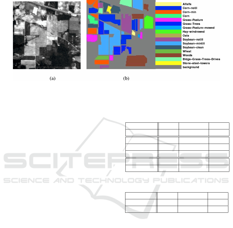
Figure 1: The Indian pines picture (a) and ground truth for the classification (b) From (Manian and Jimenez, 2007).
classifier, regardless the kernel. Moreover, the RBF
kernel yielding best results as standalone classifier (in
our experiment as well as in experiments presented in
(Melgani and Bruzzone, 2004)) is the one most im-
proved.
By comparing the classification scheme A, with
VB analysis and B, only with secondary training with
limited class set, we can see that the Second Stage A
achieves advantage over Second Stage B, though only
minimal. That suggest that the small training sample
very well reflects the whole body of the data – when
the voting sequence is the same, it usually means that
the vector class is also the same.
There is also at least 1 correct vote in over 90 per-
cent of cases (as seen in table 2), which means that
only in 10 % of cases second stage has no chances of
improving the results, since in those cases the correct
c(v) is not included in second-stage learning set. That
suggests that a scheme for choosing the right classifier
from the first stage pool could be a promising concept.
What seems to be the main downside of presented
scheme is that it is time consuming – most of the
second stage classifications require new SVM clas-
sifier trained with pool of vectors limited by the first
stage analysis. The need of possible retraining (while
it certainly lowers with greater number of train vec-
tors) would also require to have the learning dataset
available, which may be space-consuming should the
dataset be really large.
4 CONCLUSION
The addition of the second stage to classification
scheme, as well as several classifiers (with signifi-
cantly lower accuracy rate) for refinement purposes
noticeably increases the results of SVM classifier with
all three analyzed kernels.
Table 1: The accuracy achieved in the experiment - in the
first line we see one stage classification using SVM with
three different kernels, in next three lines - the results of
supporting classifiers and in the last line the accuracy by
two stages classification scheme.
Linear Polynomial RBF
Base SVM 0.6824 0.7701 0.7740
KNN 0.6776 0.6762 0.6845
DTree 0.6109 0.6100 0.6070
BN 0.5093 0.5041 0.4874
Sec. stage A 0.7142 0.7916 0.8136
Sec. stage B 0.7021 0.7887 0.8080
Table 2: The percentage of cases in which correct classifi-
cation was present in V (v).
Linear Polynomial RBF
≥ one vote 0.8136 0.84 0.9210
≥ two votes 0.8080 0.7916 0.8312
While in some cases the second stage results do
not take into consideration the correct classification
result (as it did not appear in any vote of the first
stage), these situations constitute of less than 10 per-
cent of cases. What can also be observed is that small
learning set well reflects the whole body of hyper-
spectral vectors.
What is also important, that presented two stage
scheme is not spatially enhanced (in the way as pre-
sented in (Xu and Li, 2014)). Thus, achieved results
are not to be compared to the spatially enhanced clas-
sifiers, but only to their first stage. Further refinement
of the initial classification in this manner is of course
possible.
ICPRAM 2016 - International Conference on Pattern Recognition Applications and Methods
390

ACKNOWLEDGEMENT
The work on this article has been supported by
the project ‘Representation of dynamic 3D scenes
using the Atomic Shapes Network model’ fi-
nanced by National Science Centre, decision DEC-
2011/03/D/ST6/03753.
REFERENCES
Bhaskaran, S., Datt, B., Forster, T., T., N., and Brown, M.
(2004). Integrating imaging spectroscopy (445-2543
nm) and geographic information systems for post-
disaster management: A case of hailstorm damage
in sydney. International Journal of Remote Sensing,
25(13):2625–2639.
Bioucas-Dias, J. M., Plaza, A., Dobigeon, N., Parente, M.,
Du, Q., Gader, P., and Chanussot, J. (2012). Hy-
perspectral unmixing overview: Geometrical, statis-
tical, and sparse regression-based approaches. Se-
lected Topics in Applied Earth Observations and Re-
mote Sensing, IEEE Journal of, 5(2):354–379.
Chapelle, O., Haffner, P., and Vapnik, V. (1999). Sup-
port vector machines for histogram-based image clas-
sification. Neural Networks, IEEE Transactions on,
10(5):1055–1064.
Chen, Y., Nasrabadi, N. M., and Tran, T. D. (2013). Hy-
perspectral image classification via kernel sparse rep-
resentation. Geoscience and Remote Sensing, IEEE
Transactions on, 51(1):217–231.
Denoyer, L. and Gallinari, P. (2004). Bayesian network
model for semi-structured document classification. In-
formation Processing & Management, 40(5):807 –
827.
Ellis, J. (2003). Hyperspectral imaging technologies key for
oil seep/oil-impacted soil detection and environmental
baselines. Environmental Science and Engineering.
Retrieved on February, 23:2004.
Fang, L., Li, S., Kang, X., and Benediktsson, J. A. (2015).
Spectral–spatial classification of hyperspectral images
with a superpixel-based discriminative sparse model.
Geoscience and Remote Sensing, IEEE Transactions
on, 53(8):4186–4201.
Friedl, M. and Brodley, C. (1997). Decision tree classifica-
tion of land cover from remotely sensed data. Remote
Sensing of Environment, 61(3):399 – 409.
Kuncheva, L. (2002). A theoretical study on six classifier
fusion strategies. Pattern Analysis and Machine Intel-
ligence, IEEE Transactions on, 24(2):281–286.
Kuncheva, L., Bezdek, J., and Duin, R. (2001). Decision
templates for multiple classifier fusion: an experimen-
tal comparison. Pattern Recognition, 34:299–314.
Manian, V. and Jimenez, L. O. (2007). Land cover and ben-
thic habitat classification using texture features from
hyperspectral and multispectral images. Journal of
Electronic Imaging, 16(2):023011–023011–12.
Melgani, F. and Bruzzone, L. (2004). Classification of hy-
perspectral remote sensing images with support vec-
tor machines. Geoscience and Remote Sensing, IEEE
Transactions on, 42(8):1778–1790.
Perrone, M. P. and Cooper, L. (1993). When networks dis-
agree: Ensemble methods for hybrid neural networks.
pages 126–142. Chapman and Hall.
Pu, Y.-Y., Feng, Y.-Z., and Sun, D.-W. (2015). Re-
cent progress of hyperspectral imaging on quality and
safety inspection of fruits and vegetables: A review.
Comprehensive Reviews in Food Science and Food
Safety, 14(2):176–188.
Rojas, M., D
´
opido, I., Plaza, A., and Gamba, P. (2010).
Comparison of support vector machine-based pro-
cessing chains for hyperspectral image classification.
In SPIE Optical Engineering+ Applications, pages
78100B–78100B. International Society for Optics and
Photonics.
Ruta, D. and Gabrys, B. (2000). An overview of classifier
fusion methods.
Wolpert, D. (1992). Stacked generalization. Neural Net-
works, 5:241–259.
Xu, L. and Li, J. (2014). Bayesian classification of hyper-
spectral imagery based on probabilistic sparse repre-
sentation and markov random field. Geoscience and
Remote Sensing Letters, IEEE, 11(4):823–827.
Two Stage SVM Classification for Hyperspectral Data
391