Earth Rotation: An Example to Teach Rigid Body Motion

and Environmental Monitoring

A Fallout of the Exploitation of LARES Satellite Data

Antonio Paolozzi

1,3

, Erricos Pavlis

, Claudio Paris

3,1

, Giampiero Sindoni

and Ignazio Ciufolini

4,3

Scuola di Ingegneria Aerospaziale, Sapienza University of Rome, Via Salaria 851-881, 00138 Rome, Italy

Joint Center for Earth Systems Technology, (JCET/UMBC), University of Maryland,

1000 Hilltop Circle, Baltimore, Maryland, 21250, U.S.A.

Museo Storico della Fisica e Centro Studi e Ricerce Enrico Fermi, Via Panisperna, 89, 00184, Rome, Italy

Dipartimento di Ingegneria dell’Innovazione Università del Salento, Via per Monteroni, 73100, Lecce, Italy

Keywords: Earth Rotation, Gravitation, Environmental Changes, Satellite Laser Ranging.

Abstract: The use of satellite laser ranging in combination with other space geodetic techniques allows us to determine

Earth’s motion with unprecedented accuracy, which is not as simple as usually described in basic textbooks.

Besides rotation and revolution there is a wobble of the rotation axis that can be derived by the torque free

case in rigid body dynamics. The presence of gravitational perturbations complicates the motion and

considering Earth as non-rigid introduces even more variations in the basic Earth motion theory. What is

interesting is that also the mass redistribution of air and water on the planet can affect the motion of Earth’s

rotational axis. Thanks to the millimetre accuracy achievable today, it is possible to correlate very small

anomalous rotational axis displacements with global environmental changes such the change in ice melting.

The paper will show the experimental motion of the Earth rotation axis and interpret it with the use of the

Euler rigid body equations of motion, outlining also the effects of the gravitational perturbations of other

bodies in the solar system and of the global climate changes on the Earth rotational axis.

1 INTRODUCTION

The Earth rotation is more complicated than what

non-specialists could think, although the main

components of the motion are sufficiently intuitive.

Before the advent of space age it was not possible to

test appropriately freely rotating bodies, so the

planetary motion was the best paradigm available.

In the paper it will be first considered the Earth

as a rigid body so that part of the wobble of the

rotation axis will be explained using rigid body

motion equations: the Euler equations. Incidentally

we recall that the solution provided by Euler is still

valid in the limit case of the rigid Earth. The new

techniques available today can position the Earth

rotation axis with accuracies at the level of one

millimetre. Among those, laser ranging to LARES-

type satellites gives a fundamental contribution.

LARES is an Italian Space Agency (ASI) funded

program with the aim to improve the measurement of

frame dragging or Lense-Thirring effect (Ciufolini et

al., 2012a) from about 10% obtained in (Ciufolini and

Pavlis, 2004) down at the level of 1% (Ciufolini et al.

2012b). The measurement of this effect is of great

interest among scientists. Under development is the

GINGER (Gyroscopes IN GEneral Relativity)

experiment (Bosi, 2011, di Virgilio, 2014). The

apparatus will exploit the Sagnac effect in the ring-

lasers to measure frame-dragging.

Contrary to the above missions, LARES is instead

a completely passive satellite so it is intrinsically

simpler and more reliable. It is covered with Cube

Corner Reflectors (CCRs) that have the property of

reflecting laser pulses sent from the ground stations

of the International Laser Ranging Service (Pearlman

et al., 2002). Counting the return time of the pulses

one determines the satellite position with few

millimetres accuracy.

The accurate reconstruction of the orbit not only

is useful for fundamental physics but also for the

accurate determination of the position of the centre of

mass and rotation axis of the Earth (in one word of

the Earth reference frame). The feasibility of

Paolozzi, A., Pavlis, E., Paris, C., Sindoni, G. and Ciufolini, I.

Earth Rotation: An Example to Teach Rigid Body Motion and Environmental Monitoring - A Fallout of the Exploitation of LARES Satellite Data.

In Proceedings of the 8th International Conference on Computer Supported Education (CSEDU 2016) - Volume 2, pages 339-346

ISBN: 978-989-758-179-3

339

verifying the General Relativity effect but also the

possibility of determining accurately the rotation axis

of the Earth rely not only to the high accuracy of the

orbit determination reachable with the laser ranging

technique. Other factors such as the reduction of the

effects on the non-gravitational perturbation achieved

with a special design of LARES satellite and its

estimation is mandatory, as shown in the Monte Carlo

simulations of the experiment reported in (Ciufolini

et al., 2013a).

The special design of LARES provides accurate

data that integrated with data of other satellites and

techniques allow us determine an accurate Earth

reference frame (Pavlis et al., 2015a). In particular to

reduce the non-gravitational perturbations a very high

density material (Paolozzi et al., 2009) have been

chosen for the satellite. To further reduce unmodeled

effects on the satellite orbit, radiation pressure

uncertainties have been limited by avoiding painting

the surface of the satellite. Also thermal thrust

perturbation have been minimized (Ciufolini et al.,

2014) using a different approach with respect to what

originally proposed in (Bosco et al., 2007) i.e.

reducing the main origin of this perturbation: the

CCRs. The surface of the CCRs as compared to the

metallic surface of the satellite is the lowest with

respect to what obtained in all other laser-ranged

satellites (Ciufolini et al., 2013b; Paolozzi et al.,

2015).

February 13, 2012 LARES was successfully put

in orbit with the VEGA launcher (Paolozzi et al.,

2013; Paolozzi et al., 2012b) and data analysis for

testing General Relativity is now in progress

(Ciufolini et al., 2015).

In this paper we will concentrate on Earth’s

rotation axis showing that most of its motion can be

explained by rigid body dynamics. Relation with

climate change is also pointed out and indeed the

combination of mechanics and environmental

monitoring is believed to be an excellent driver to

raise students’ interest in both fields.

2 PLANETARY MOTION

In basic textbooks it is reported that planets, and in

particular the Earth, have two main motions:

revolution, which follows the second Kepler law

(equal areas are swept out in equal time) and rotation

characterized by a spin axis and angular velocity

(considered both constant at first approximation). It is

interesting to observe that those two motions are

easily predictable under two simplified assumptions:

• Rigid body Earth

• External actions limited to conservative

central forces.

If one neglects the non-gravitational perturbations

and the gravitational actions of all the other bodies

with the exclusion of the Sun, that is the source of the

conservative central force, the second hypothesis

applies to all planets in the solar system. In this

simplified scenario the conservation law of angular

momentum provides an endless motion of the planets

according to the second Kepler law i.e. the well-

known revolution motion.

Concerning the rotation being constant in

magnitude and direction, the additional hypothesis of

the Earth being infinitely rigid is required. In fact for

a non-rigid Earth it could happen that the rotational

speed would increase as a result of a reduction of the

diameter, exactly in the same way as it would happen

to a spinning ice skater when she/he brings the arms

closer to the body. Also the direction of the rotational

axis could change if the symmetry is broken by mass

redistribution on the Earth. In the analogy of the

skater also the rotational axis would change if only

one arm is retracted. However this hypothesis is not

sufficient to guarantee that the spin axis remains

constant in inertial space. This aspect will be analyzed

in detail later in the paper.

It is customary in rigid body motion analysis to

use a reference frame fixed with the body, and this

approach is maintained here for the case of the Earth.

The Earth reference frame is defined by the

International Earth Rotation and Reference Systems

Service (IERS) and is called International Terrestrial

Reference Frame or ITRF in short. The geographic

position of the North and South poles are defined with

a complex procedure that uses several techniques

including satellite laser ranging on LARES-like

satellites. The addition of LARES by the way will

improve the accuracy of such a reference frame by

about 20% as shown in (Pavlis et al., 2015a; Sindoni

et al., 2015). The geographic location of North and

South will define a geometric axis that does not

coincide with the rotational axis of the Earth. One

could think this rotation axis of the Earth is fixed in

inertial space and consequently could be considered a

realization of an inertial reference frame. But that in

general would be a mistake even if the Earth would

be an ideal perfect gyroscope as will be shown later

in the paper.

In summary there are several reasons why the

rotation axis of the Earth cannot be fixed in inertial

space, and with respect to the ITRF:

CSEDU 2016 - 8th International Conference on Computer Supported Education

340

1) Even if the Earth would be an ideal gyroscope,

the rotation axis, in general, is not fixed in

inertial space. In fact what remains fixed in

inertial space is the angular momentum vector

(see details later in the paper). In short,

Newton’s second law, written in an inertial

reference frame, will imply the conservation of

angular momentum vector L that only under

very special situations is parallel to the angular

velocity vector ω.

2) The Earth is not a rigid body.

3) There are gravitational actions acting on the

Earth other than the solar attraction.

4) There are non-gravitational perturbations

acting on the Earth.

In the following section we recall some

fundamentals of rigid body dynamics preferring,

whenever possible under the limited space available

here, a graphical approach and pointing out some

pitfalls that usually arise in this area.

3 ANGULAR MOMENTUM

AND ANGULAR VELOCITY

First we recall that the angular momentum vector L is

a quantity that depends on the rotation speed of the

body, and on the mass distribution of the body itself

with respect to three arbitrary axes. The angular

velocity vector of the body ω is measured in a chosen

reference frame (usually an inertial frame, but not

necessarily). The mass distribution is summarized by

six independent numbers that are collected in a

symmetric matrix called the matrix of inertia I also

defined in an arbitrary reference frame (usually the

body fixed reference frame). In compact form the

rigorous definition of angular momentum in a

reference frame where the body is “seen” to rotate

with an angular velocity ω is:

L=Iω

(1)

If the reference frame, where ω is measured, is an

inertial reference frame and there are no torques

applied to the body, the vector L does not change

(conservation of angular momentum) so that in

general if ω changes in direction and/or magnitude

also I need to change to maintain L constant in time.

The change of I is difficult to deal with so one can

considerer at each instant an inertial reference frame

that is aligned with the body reference frame and

centred in the centre of mass of the body. In this series

of inertial reference frames the above equation holds,

meaning the L is constant although its components

change in time because the reference frame is

changing. If, in addition, we take the axes of those

inertial reference frames parallel to the principal axes

of inertia of the body (in general for regular shaped

object those coincide with the symmetry axes), then

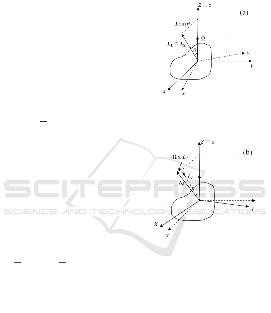
the matrix I becomes diagonal. In Figure 1 the

situation is depicted.

Figure 1: (a) Inertial reference frame at instant t=t

; (b)

Inertial reference frame, rotated with respect to (a), at

instant t=t

. Vector L is the same as in (a) (conservation of

angular momentum) but its components have changed.

For the sake of clarity only x and y components of L

have been represented. Note that L has not changed

(conservation of angular momentum) from Figures 1a

to Figure 1b, while its components on the rotated

reference frame have changed. Also ω from time t

(Figure 1a) and time t

(Figure 1b) has changed. Also

note that in general L and ω are not parallel in this

series of inertial reference frames.

There are however special cases in which the two

vectors L and ω are parallel:

a) All three components of moments of inertia are

equal, i.e.

=





0



00





(2)

with I

=I.

(a)

Earth Rotation: An Example to Teach Rigid Body Motion and Environmental Monitoring - A Fallout of the Exploitation of LARES Satellite

Data

341

In this case Eq. 1 reduces to L=Iω, i.e. the two

vectors differ in magnitude by the factor given

by the moment of inertia I.

b) Only one component of vector ω is different

from zero, with the exclusion of the component

corresponding to the direction of the

intermediate moment of inertia (because of

instability of rotation around the intermediate

axis) i.e. suppose I

then it can be

=ω

=0 or ω

=ω

=0. In this last case one has:

=0 and L

In both cases ω is conserved and this fact let

erroneously think that this is a general law, which is

not, since what is conserved in torque free motion and

in an inertial reference frame is the angular

momentum vector and not the angular velocity

vector.

As an example of the fact that the two vectors are

not parallel let us consider the Earth. Using updated

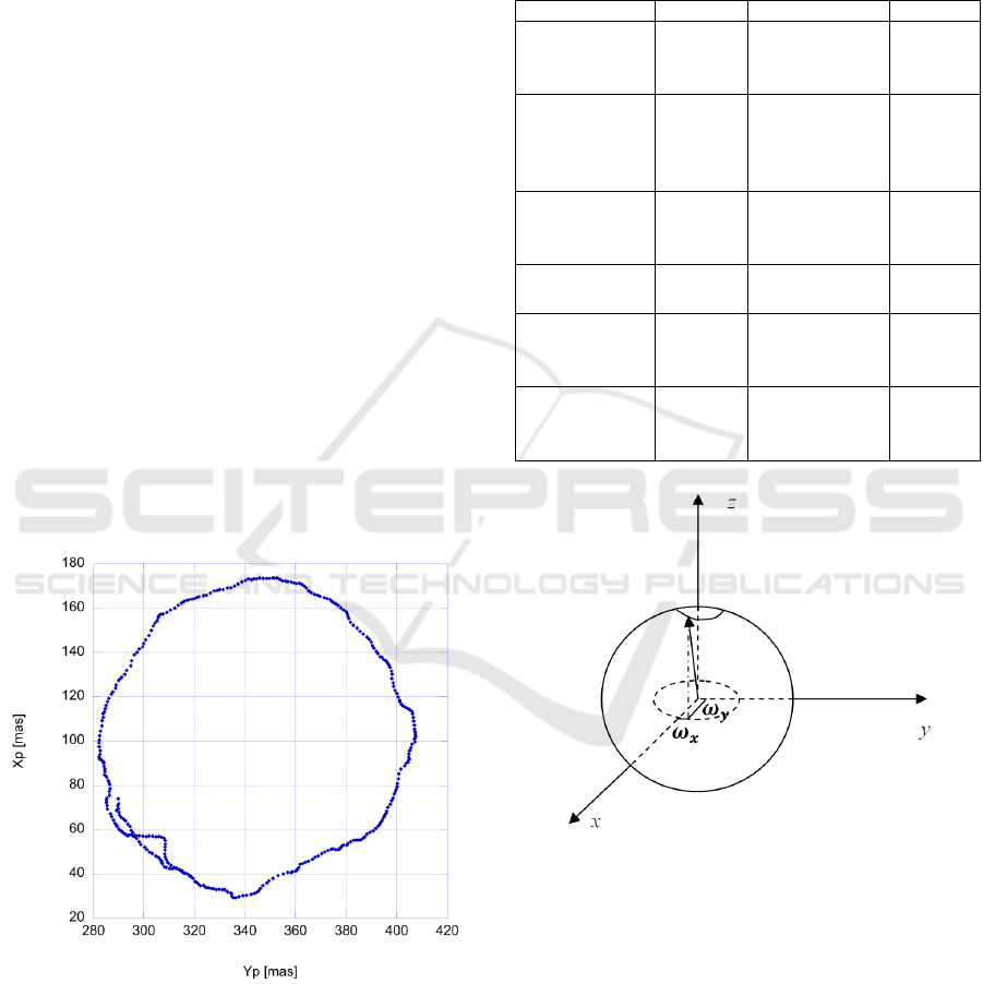
data from LARES satellite, in Figure 2 is reported the

actual motion of the Earth axis in year 2013 as seen

from the ITRF. The motion shown in Figure 2 proves

that L and ω are not parallel. In fact the Earth is not

perfectly spherical as shown by the values reported in

Table 1 (thus point (a) above does not apply) and ω

has components, though extremely small, also along

the two horizontal axes of the ITRF (thus point (b)

above does not apply).

Figure 2: Track of the Earth rotation axis with the Earth

surface as seen from an observer over the North pole and

fixed in the ITRF. The figure refers to year 2013 and has

been obtained including LARES data. 1 milliarcsecond

(mas) corresponds approximately to 3 cm on the Earth’s

surface.

In Figure 3 is reported a sketch where the diameter of

the trajectory of Figure 2 has been magnified by a

factor of about 10

Table 1: Earth’s moments of inertia. Uncertainty on last

digit in parenthesis. (from http://hpiers.obspm.fr/eop-

pc/models/constants.html#chenshen).

Constant Symbol Value Unit

First equatorial

moment of

inertia

8.0101 (2)

kg m

Second

equatorial

moment of

inertia

8.0103 (2)

kg m

Mean equatorial

moment of

inertia

mean

)/2

8.010171 (84)

kg m

Axial moment

of inertia

8.0365 (2)

kg m

Mean angular

velocity of the

Earth

Ω 7.2921150 (1) 10

-5

rad/s

First equatorial

moment of

inertia

8.0101 (2)

kg m

Figure 3: Trajectory (out of scale) of ω vector in the body

fixed reference frame.

4 EQUATIONS OF RIGID

BODY MOTION

What is causing the wobble reported in Figure 2 and

Figure 3? At the beginning of the paper we listed four

possible causes of the movement of the rotation axis

of the Earth. It is reasonable to expect all of them

contributing to this unexpected movement. Referring

to point 2 for instance one can refer to (Creveling J.R.

CSEDU 2016 - 8th International Conference on Computer Supported Education

342

et al., 2012). But what is the major contributor for the

Earth axis rotation? We will see, in the relatively

straightforward derivations below, that this wobble is

mainly due to the most basic law of mechanics: F=ma

(with F=0) applied as a total moment to a rigid body.

Euler calculated this effect, with a period of about 305

days, back in 1765. The actual experimental value

was observed by Chandler as being of about 439 days.

The discrepancy was later explained by Newcomb by

the fact that the Earth is not rigid (point 2 at beginning

of paper). But there are also other effects contributing

to this motion as will be mentioned at the end of the

paper.

Euler second law in an inertial reference frame

states that the rate of change of angular momentum

equates the applied torque T:











=

(3)

But as mentioned earlier it is convenient to use a body

fixed reference frame. So how the previous law will

change? To make the graphical representation more

understandable let us consider t=0 so that angular

momentum conservation applies and L is therefore

constant. in the body fixed reference frame an

observer would see the vector L changing direction

(Figure 4). It is easy to see that the rate of change of

L is given by Ω L sinθ, or using the vector product

notation, -Ω×L where Ω is the angular velocity vector

of the body fixed reference frame with respect to an

inertial reference frame and ω is the angular velocity

magnitude. What described is a transformation valid

for calculating the rate of change of any vector in two

rotating reference frames. So the rate of change of a

vector, and in particular of L, as seen from a body

fixed reference frame is:











=









−×

(4)

Note: it is useful to observe something that is obvious

but that sometimes is confusing. Vector Ω is

measured in the inertial reference frame. Instead the

angular velocity as measured from the body fixed

reference frame, i.e. the one of the inertial frame with

respect to the body frame, is Ω

from_body

= - Ω. It is also

useful to note that those two angular velocities do

exist in their respective reference frames. Although

the angular velocity Ω of the relative rotation of the

two reference frames equals the angular velocity of

the body ω, the two quantities are conceptually

different. In fact ω would be zero as measured from

the body fixed reference frame while in this frame the

angular velocity of the inertial frame with respect to

the body frame Ω

from_body

is equal to – Ω.

Figure 4a: Vector L as seen from the inertial reference

frame (solid line). The body fixed reference frame rotates

with angular velocity Ω. At time t

it is in the position

shown by the dashed lines. Subscripts correspond to the

time t

and t

Figure 4b: Vector L as seen from the body fixed reference

frame (dashed line). An observer on the moving frame would

see the inertial frame rotate in opposite direction so that at t

it will be as shown by the solid lines. The rate of change of L

is due to the rotation of the axes and is -Ω×L

or to

Ω

from_body

×L

. Subscripts correspond to the time t

and t

Rewriting Equation 4 in the general case of torque T

different from zero we have:











=









+×

=

(5)

Recalling that the inertia matrix I, in the body fixed

reference frame, does not change, the definition of L

from Equation 1 and that Ω=ω (remembering the note

reported above) we obtain the Euler equation for rigid

body motion in vector form:

∙



+×



∙



(6)

Earth Rotation: An Example to Teach Rigid Body Motion and Environmental Monitoring - A Fallout of the Exploitation of LARES Satellite

Data

343

Having chosen the body axis aligned with the inertia

principal axis, the above equation becomes:







0



00

















+















×





0



00



















=















(7)

By performing the simple calculations one obtains the

Euler equations:









−











−



=











−













−





=











−











−



=



(8)

Now in the case of the Earth, if we neglect the

external actions and the very small differences

between I

and I

, the above equations simplifies to:









=











−













=−













−













(9)

with the third equation providing ω

=constant.

Furthermore by posing:

Ω







−











(10)

and substituting the values reported in Table 1 one

obtains:

Ω



8.0365−8.0102

8.0102

7.2921∙10







=2.3942∙10







=3.294∙10









(11)

This angular frequency corresponds to a period of

303.6 days and the above equations reduce to:





=−Ω











=Ω







(12)

The solution to this system of linear differential

equations can be easily verified to be:







cosΩ











sinΩ





(13)

In the x-y plane of the body reference frame the

projection of the vector ω will trace in a period of

303.6 days a circle similar to that depicted with

dashed line in Figure 3.

So we have shown that a rotating body with no

external torques does not have, in general, a rotation

axis fixed in inertial space and with respect to the

body fixed reference frames. This last motion is

referred to as polar motion. Incidentally we observe

that it is still not clear what maintains the wobble

against the viscoelastic damping of the interior of the

Earth (Jenkins, 2015).

5 OTHER EFFECTS

AND ENVIRONMENTAL

MONITORING.

In this section we will briefly assess the effects of

points 2 and 3 mentioned at the beginning of the

paper.

We have mentioned that the polar motion is a

combination of several effects. The main one has

been described in the previous section and is due to

the law of mechanics applied to a torque free rigid

body. If we add the non-rigid Earth component, the

resulting wobble period would change from 303.6

days to about 439 days which is approximately the

value measured by Chandler. A more accurate

inspection of the motion over a longer period of time

will reveal that the radii of the circles (one is shown

in Figure 2), varies from about 3 meters to about 15

meters over a 6.5 year period. This variation cannot

be simply explained with the torque free motion and

the non-rigidity of the Earth because it is due to some

external seasonal forcing action that has a period of

one year.

But besides the wobbles just described there are

other components on the motion of the rotation axis

of the Earth. The effects of the gravitational torques

mainly of the Moon and the Sun, on the equatorial

bulge of the Earth causes the rotational axis of the

Earth to precess with a period of 25700 years. This

phenomenon is analogous to the precession of a

spinning top. Furthermore since the positions of the

Moon and the Sun change with time this effect

produces a nutation i.e. an oscillation of the Earth spin

axis with main period of 18.6 years (lunisolar

precession). Also the gravitational perturbations of

the planets induce a change of inclination of the Earth

axis in the range 22.2 – 24.3 degrees with a mean

period of 41.000 years (Berger A.L., 1976).

Possible indications on climate change can be

inferred by additional Earth rotation axis shift (Roy

and Peltier, 2011; Pavlis et al., 2015b). In fact mass

CSEDU 2016 - 8th International Conference on Computer Supported Education

344

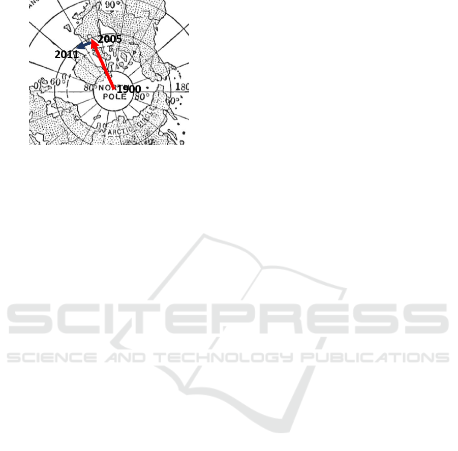
Figure 5: The long arrow (from year 1900 to 2005)

corresponds to 12.6m, the short arrow (from 2005 to 2011)

is of 1.6 m.

redistribution inside or on the surface of the planet

will affect the Length of the Day (LOD) and the

rotation axis direction (in one sentence, the angular

velocity vector) similarly to what would happen to the

skater mentioned above when he/she moves the arms.

The mass redistribution on the surface of the planet

concerns the atmosphere, the glaciers (Cazenave, A.,

and Chen J.L. 2010), the oceans, etc… We just would

like to mention another small motion of the rotation

axis of the Earth that is a secular drift towards East

which is partly due to post-glacial rebound i.e. the

slow ground rise due to the recovery of the original

position of the ground after the melting, and

consequently the release of weight, of the enormous

quantity of glaciers produced during the ice age. In

2005 it was observed a sudden change of the direction

of this secular drift that is attributed to a rapid melting

of Greenland glaciers and polar caps (Figure 5) (Chen

et al., 2013). Also the El Niño, due to thermal

expansion of the Pacific ocean (about 20 cm sea level

rise for an extension of thousands of kilometers)

produces variation on the Earth Orientation

Parameters (EOP) i.e. LOD and rotation axis

direction. The variations are very small but the

accuracy reached with the laser ranging technique on

LARES and other geodetic satellites and other

methods such as GNSS and Very Long Baseline

Interferometry (VLBI) allow to monitor the axis

position with an error of the order of 0.03

milliarcsecond i.e. about 1 mm on the Earth surface.

6 CONCLUSIONS

Taking the planet Earth as an example for a rotating

body, the paper describes first the case in which the

Earth is considered infinitely rigid. In this limit case

the rigid body Euler equations of motion predict a

counterintuitive oscillation of the Earth rotation axis,

that is the main contributor to the so called Chandler

wobble. This oscillation is a remarkable case because

it is not due to external torques but simply to the laws

of mechanics for a freely rotating body. The

discrepancy of the period of the wobble obtained

experimentally by Chandler with what obtained by

the Euler equations is explained with the non-rigid

Earth. Other motions of the axis are due to external

gravitational actions of the planets and particularly of

the Moon and the Sun. Finally the correlation

between the variation on the angular velocity vector

or if you like on the Earth Orientation Parameters

(EOP) and global climate changes is outlined. In

particular it has been observed that rapid Greenland

and polar ice melting may be the cause of the sudden

change in the polar motion secular drift. Also the

Pacific Ocean thermal expansion of El Niño

frequently leaves a signature on the EOP. Besides

being important for research in the field of global

climate change monitoring, Earth rotation studies

have recently gained considerable interest with the

public, mainly thanks to the proliferation of the web

and the increased outreach efforts of all scientists.

The combination of two fields, climatology and

mechanics, that appear to be so far apart seems to

attract very much the interest probably due to the

increasing concern on environmental issues. We plan

to apply this approach of combining mechanics, Earth

rotation and global environmental monitoring in an

educational and public outreach context to verify its

validity.

ACKNOWLEDGEMENTS

Research on the LARES mission is supported by the

Italian Space Agency under contracts I/034/12/0,

I/034/12/1, and 2015-021-R.0. E. C. Pavlis

acknowledges the support of NASA Grants

NNX09AU86G and NNX14AN50G. The authors

thank the International Laser Ranging Service for

tracking LARES and providing the laser ranging data.

REFERENCES

Berger A. L., 1976. Obliquity and Precession for the Last

5.000.000 Years. Astron. & Astrophys., 51, 127-135.

Bosi F., et al., 2011. Measuring gravito-magnetic effects by

multi ring-laser gyroscope. Phys. Rev. D. vol. 84, p.

122002-1-23.

Earth Rotation: An Example to Teach Rigid Body Motion and Environmental Monitoring - A Fallout of the Exploitation of LARES Satellite

Data

345

Bosco, A., Cantone, C., Dell'Agnello, S., Delle Monache,

G. O., Franceschi, M. A., Garattini, M., et al., 2007.

Probing gravity in NEO with high-accuracy laser-

ranged test masses. International Journal of Modern

Physics D, vol. 16, p. 2271-2285.

Cazenave, A., and Chen J. L., 2010, Time-variable gravity

from space and present-day mass redistribution in the

Earth system, Earth and Planetary Science Letters,

298, 263–274.

Chen, J. L., Wilson, C. R., Ries, J. C., Tapley, B. D., 2013.

Rapid ice melting drives Earth’s pole to the east,

Geophysics Research Letters, 40, 2625–2630.

Ciufolini, I. and Pavlis E. C., 2004. A confirmation of the

general relativistic prediction of the Lense-Thirring

effect. Nature 431, 958–960.

Ciufolini, I., Pavlis, E. C., Paolozzi, A., Ries, J., Koenig, R.,

Matzner, R., Sindoni, G., Neumayer H., 2012a.

Phenomenology of the Lense-Thirring effect in the

Solar System: Measurement of frame-dragging with

laser ranged satellites. New Astronomy, 17(3), 341-346.

Ciufolini, I., Paolozzi, A., Paris, C., 2012b. Overview of the

LARES Mission: orbit, error analysis and technological

aspects. Journal of Physics, Conference Series, vol.

354, p. 1-9.

Ciufolini, I., Moreno Monge, B., Paolozzi, A., Koenig, R.,

Sindoni, G., Michalak G., Pavlis, E. C., 2013a. Monte

Carlo simulations of the LARES space experiment to

test General Relativity and fundamental physics.

Classical and Quantum Gravity, 30, 235009.

Ciufolini, I., Paolozzi, A., Koenig, R., Pavlis, E. C., Ries,

J., Matzner, R., Gurzadyan, V., Penrose, R., Sindoni,

G., Paris, C., 2013b. Fundamental Physics and General

Relativity with the LARES and LAGEOS satellites.

Nuclear Physics B-Proceedings Supplements, vol. 243-

244, p. 180-193.

Ciufolini, I., Paolozzi, A., Paris, C., Sindoni, G., 2014. The

LARES satellite and its minimization of the thermal

forces. In: IEEE International Workshop on Metrology

for Aerospace. Conference Proceedings, pp. 299-303.

IEEE.

Ciufolini, I., Paolozzi, A., Pavlis, E. C., Koenig, R., Ries,

J., Gurzadyan, V., Matzner, R., Penrose, R., Sindoni,

G., Paris, C., 2015. Preliminary orbital analysis of the

LARES space experiment. The European Physical

Journal Plus, vol. 130.

Creveling, J. R., J. X. Mitrovica, N.-H. Chan, K. Latychev,

and I. Matsuyama (2012), Mechanisms for oscillatory

true polar wander, Nature, 491, 244–248.

Di Virgilio, A., Allegrini, A., Beghi, M., Belfi, A., et al.,

2014. A ring lasers array for fundamental physics.

Comptes Rendus Physique, vol. 15, p. 866-874.

Jenkins, A., 2015. On the maintenance of the Chandler

wobble. arXiv:1506.02810v1 [physics.geo-ph], 9 Jun,

2015.

Paolozzi, A., Ciufolini, I., Felli, F., Brotzu, A., Pilone, D.,

2009. Issues on lares satellite material. In: Proceedings

of International Astronautical Congress IAC 2009,

Daejeon, Republic of Korea.

Paolozzi, A., Ciufolini, I., Flamini, E., Gabrielli, A.,

Pirrotta, S., Mangraviti, E., Bursi, A., 2012. LARES in

orbit: some aspects of the mission. Proceedings of

Inter, Astronautical Congress IAC 2012

, Naples, Italy.

Paolozzi, A., Ciufolini, I., 2013. LARES successfully

launched in orbit: satellite and mission description.

Acta Astronautica, vol. 91, pp. 313-321.

Paolozzi, A., Ciufolini, I., Paris, C., Sindoni, G., 2015.

LARES a new satellite specifically designed for testing

general relativity. International Journal of Aerospace

Engineering, vol. 2015, p. 1-10.

Pavlis, E. C., Ciufolini, I., Paolozzi, A., Paris, C., Sindoni,

G., 2015a. Quality assessment of LARES satellite

ranging data. LARES contribution for improving the

terrestrial reference frame. In: 2nd IEEE International

Workshop on Metrology for Aerospace. Conference

Proceedings. vol. 1, p. 33-37. IEEE.

Pavlis, E. C., Sindoni, G., Paolozzi, A., Ciufolini, I., 2015b.

Contribution of LARES and Geodetic Satellites on

Environmental Monitoring. Proc. of 15th IEEE

International Conference on Environment and

Electrical Engineering - IEEE EEEIC 2015. IEEE.

Pearlman, M. R., Degnan, J. J. and Bosworth, J. M., 2002.

The International Laser Ranging Service. Advances in

Space Research, 30, pp. 135-143.

Roy, K., and Peltier W. R., 2011. GRACE era secular trends

in Earth rotation parameters: A global scale impact of

the global warming process?. Geophysics Research

Letters, 38, L10306, pp.1-5.

Sindoni, G., Paris, C., Vendittozzi, C., Pavlis, E. C.,

Ciufolini, I., Paolozzi A., 2015. The contribution of

LARES to global climate change studies with geodetic

satellites. Proc. of the ASME 2015 Conference on Smart

Materials, Adaptive Structures and Intelligent Systems

SMASIS 2015. ASME.

CSEDU 2016 - 8th International Conference on Computer Supported Education

346