A Hadoop based Framework to Process Geo-distributed Big Data

Marco Cavallo, Lorenzo Cusma’, Giuseppe Di Modica, Carmelo Polito and Orazio Tomarchio

Department of Electrical, Electronic and Computer Engineering, University of Catania, Catania, Italy

Keywords:

Big Data, Mapreduce, Hierarchical Hadoop, Context Awareness, Integer Partitioning.

Abstract:

In many application ﬁelds such as social networks, e-commerce and content delivery networks there is a con-

stant production of big amounts of data in geographically distributed sites that need to be timely elaborated.

Distributed computing frameworks such as Hadoop (based on the MapReduce paradigm) have been used to

process big data by exploiting the computing power of many cluster nodes interconnected through high speed

links. Unfortunately, Hadoop was proved to perform very poorly in the just mentioned scenario. We de-

signed and developed a Hadoop framework that is capable of scheduling and distributing hadoop tasks among

geographically distant sites in a way that optimizes the overall job performance. We propose a hierarchi-

cal approach where a top-level entity, by exploiting the information concerning the data location, is capable

of producing a smart schedule of low-level, independent MapReduce sub-jobs. A software prototype of the

framework was developed. Tests run on the prototype showed that the job scheduler makes good forecasts of

the expected job’s execution time.

1 INTRODUCTION

Big data technologies have appeared in the last decade

to serve the growing need for computation in all the

ﬁelds where old data mining techniques did not suite

anymore because of the really big size of the data

to be analyzed. First problem to face when coming

across big data computation is where to put data. The

Cloud has been evoked by many as the right place

where data ought to be stored and mined (Wright and

Manieri, 2014). The Cloud can scale very well with

respect to both the data dimension and the computing

power that is required for elaboration purposes. Be-

cause of the huge data dimension, moving the com-

putation close to the data seems to be the most smart

and advisable strategy. Nevertheless, the assumption

that data are concentrated in just one place does not

always hold true. On the contrary, in many applica-

tions very frequently data are conveyed to data cen-

ters which are geographically distant to each other’s

(Petri et al., 2014).

Application parallelization and divide-and-

conquer strategies are natural computational

paradigms for approaching big data problems,

addressing scalability and high performance. The

availability of grid and cloud computing technolo-

gies, which have lowered the price of on-demand

computing power, have spread the usage of parallel

paradigms, such as the MapReduce (Dean and Ghe-

mawat, 2004), for big data processing. However, in

scenarios where data are distributed over physically

distant places the MapReduce technique may perform

very poorly. Hadoop, one of the most widespread

implementation of the MapReduce paradigm, was

mainly designed to work on clusters of homogeneous

computing nodes belonging to the same local area

network; thus, data locality is one of the crucial

factors affecting its performance. Tests run on a

geographic test-bed have proved that the time for

a Hadoop job to complete uncontrollably increases

because the shifts of data triggered by the algorithm

are penalized by the low speed geographic links.

This work discusses the design and implementa-

tion of a software system conceived to serve MapRe-

duce jobs that need run on geo-distributed data. The

proposed solution follows a hierarchical approach,

where a top-level entity takes care of serving a

submitted job: the job is split into a number of

bottom-level, independent MapReduce sub-jobs that

are scheduled to run on the sites where data natively

reside or have been ad-hoc moved to. The designed

job scheduling algorithm aims to exploit fresh in-

formation continuously sensed from the distributed

computing context (available sites computing capac-

ity and inter-site bandwidth) to estimate each jobs best

execution path. In the paper we disclose some details

on the job scheduling algorithm and, in particular, we

stress on its capability to compute the best execution

178

Cavallo, M., Cusma’, L., Modica, G., Polito, C. and Tomarchio, O.

A Hadoop based Framework to Process Geo-distributed Big Data.

In Proceedings of the 6th International Conference on Cloud Computing and Services Science (CLOSER 2016) - Volume 1, pages 178-185

ISBN: 978-989-758-182-3

path and forecast the job’s completion time. Tests

have been conducted on the software prototype in or-

der to check that the actual job’s completion time (the

one measured at job execution time) gets close to the

forecast.

The paper is organized as follows. In Section 2

the literature is reviewed. In Section 3 an overview of

the proposal is presented. Technical details of the pro-

posed system architecture are discussed in Section 4.

In Section 5 we delve into the strategy implemented

by the job scheduler component. In Section 6 the re-

sults of the tests run on the system’s software proto-

type are presented. Section 7 concludes the work.

2 RELATED WORK

In the literature two main approaches are followed

by researchers to efﬁciently process geo-distributed

data: a) enhanced versions of the plain Hadoop im-

plementation which account for the nodes and the

network heterogeneity (Geo-hadoop approach); b) hi-

erarchical frameworks which gather and merge re-

sults from many Hadoop instances locally run on dis-

tributed clusters (Hierarchical approach). The for-

mer approach aims at optimizing the job performance

through the enforcement of a smart orchestration of

the Hadoop steps. The latter’s philosophy is to exploit

the native potentiality of Hadoop on a local base and

then merge the results collected from the distributed

computation. In the following a brief review of those

works is provided.

Geo-hadoop approaches reconsider the phases of

the job’s execution ﬂow (Push, Map, Shufﬂe, Reduce)

in a perspective where data are distributed at a geo-

graphic scale, and the available resources are not ho-

mogeneous. In the aim of reducing the job’s aver-

age makespan, phases and the relative timing must be

adequately coordinated. Some researchers have pro-

posed enhanced version of Hadoop capable of opti-

mizing only a single phase (Kim et al., 2011; Mattess

et al., 2013). Heintz et al.(Heintz et al., 2014) analyze

the dynamics of the phases and address the need of

making a comprehensive, end-to-end optimization of

the job’s execution ﬂow. To this end, they present an

analytical model which accounts for parameters such

as the network links, the nodes capacity and the ap-

plications proﬁle, and transforms the makespan mini-

mization problem into a linear programming problem

solvable with the Mixed Integer Programming tech-

nique.

Hierarchical approaches tackle the problem from

a perspective that envisions two (or sometimes more)

computing levels: a bottom level, where several plain

MapReduce computations occur on local data only,

and a top level, where a central entity coordinates the

gathering of local computations and the packaging of

the ﬁnal result. In (Luo et al., 2011) authors present a

hierarchical MapReduce architecture and introduces

a load-balancing algorithm that makes workload dis-

tribution across multiple clusters. The balancing is

guided by the number of cores available on each clus-

ter, the number of Map tasks potentially runnable at

each cluster and the nature (CPU or I/O bound) of the

application. The authors also propose to compress

data before their migration from one data center to

another. Jayalath et al.(Jayalath et al., 2014) make an

exhaustive analysis of issues concerning the execution

of MapReduce on geo-distributed data. The particular

context addressed by authors is the one in which mul-

tiple MapReduce operations need to be performed in

sequence on the same data.

With respect to the cited works, our places among

the hierarchical ones. The approach we propose dif-

fers in that it strives to exploit fresh information con-

tinuously sensed from the distributed computing con-

text (available sites computing capacity and inter-site

bandwidth) and calls on the integer partitioning tech-

nique to compose the space of the job’s potential exe-

cution paths and seek for the best.

3 SYSTEM DESIGN

According to the MapReduce paradigm, a generic

computation is called “job”. Upon a job submis-

sion, a scheduling system is responsible for splitting

the job in several tasks and mapping them to a set of

available nodes within a cluster. The performance of

a job execution is measured by its completion time

(some refers to it with the term makespan), i.e., the

time for a job to complete. Apart from the size of

the data to be processed, that time heavily depends on

the jobs execution ﬂow determined by the schedul-

ing system and the computing power of the cluster

nodes where the tasks are actually executed. In a

scenario where computing nodes reside in distributed

clusters that are geographically distant to each oth-

ers, there is an additional parameter that may affect

the job performance. Communication links among

clusters (inter-cluster links) are often inhomogeneous

and have a much lower bandwidth than communica-

tion links among nodes within a cluster (intra-cluster

links). Also, clusters are not designed to have simi-

lar or comparable computing capacity, therefore they

might happen to be heterogeneous in terms of com-

puting power. Third, it is not rare that the data set to

be processed are unevenly distributed over the clus-

A Hadoop based Framework to Process Geo-distributed Big Data

179

ters. So basically, if a scheduling system does not

account for this threefold unbalancement (nodes ca-

pacity, communication links bandwidth, data set dis-

tribution) the overall jobs performance may degrade

dramatically. To face these issues, we propose a hi-

erarchical MapReduce framework where a top-level

scheduling system sits on top of a bottom-level dis-

tributed computing context and is continuously kept

informed about the dynamic conditions of the under-

lying computing context. Information retrieved from

the computing context is then used to drive the gener-

ation of each jobs optimum execution ﬂow (or execu-

tion path). The basic reference scenario addressed by

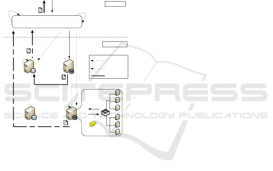
Top-Level Job

Output Data

Result

Local Hadoop Job

Top Level

Data Transfer

Top Level Manager

Execute Top-Level

MapTask

Reduce

Bottom Level

MoveData

Site1

Site3

Site2

Push Top-Level

Map Result

Site4

MapReduce

Generate TJEP

Figure 1: Job Execution Flow.

our proposal is depicted in Figure 1. Sites (data cen-

ters) populate the bottom level of the hierarchy. A Site

may be composed of one or more cluster nodes that

provide the overall Sites computing power. Each Site

stores a certain amount of data and is capable of run-

ning plain Hadoop jobs. Upon receiving a job, a Site

transparently performs the whole MapReduce process

chain on the local cluster(s) and returns the result of

the elaboration. The system business logic devoted to

the management of the geo-distributed computing re-

sides in the top-level of the hierarchy. When a new

Hadoop job is submitted that requires to process the

data distributed over the Sites, the business logic splits

the job into a set of sub-jobs, pushes them to the dis-

tributed context, gathers the sub-job results and pack-

ages the overall computation result. The novelty in-

troduced by this work is the adoption of a scheduling

strategy based on the integer partitioning technique

and the inclusion of the application proﬁle among the

parameters that may inﬂuence the jobs optimum exe-

cution ﬂow.

In the scenario of Figure 1 four geo-distributed

Sites are depicted that hold company’s business data

sets. The numbered arrows describe a typical execu-

tion ﬂow triggered by the submission of a top-level

job. This speciﬁc case envisioned a shift of data from

one Site to another one, and the run of local MapRe-

duce sub-jobs on two Sites. Here follows a step-by-

step description of the actions taken by the system to

serve the job:

1. A Job is submitted to the Top-Level Manager,

along with the indication of the data set targeted

by the Job.

2. A Top-level Job Execution Plan is generated

(TJEP). For the elaboration of this plan, infor-

mation like the distribution of the data set among

Sites, the current computing capabilities of Sites,

the topology of the network and the current capac-

ity of its links are used.

3. The Master, located in the Top-Level Manager,

send a message to Site1 in order to shift data to

Site4.

4. The actual data shift from Site1 to Site4 takes

place.

5. The Master send a message to start the sub-jobs.

In particular, top-level Map tasks are triggered to

run on Site2 and Site4 respectively. We remind

that a top-level Map task corresponds to a Hadoop

sub-job.

6. Site2 and Site4 executes local Hadoop jobs on

their respective data sets.

7. Results obtained from local execution are sent to

the Top-Level Manager.

8. The Global Reducer of the Top-Level Manager

performs the reduction of partial data.

9. Final result is returned to the Job submitter.

The whole job execution process is totally transparent

to the submitter, who just needs to provide the type

of job to execute and the location of the target data to

process.

4 SYSTEM ARCHITECTURE

The System was designed according to the Service-

Oriented-Architecture (SOA) architectural pattern.

The middleware implementation is based on the OSGi

framework (OSGi Alliance, 2013), that allows to cre-

ate a service platform for the Java programming lan-

guage and implements a complete and dynamic com-

ponent model. Each component, conﬁgured as an

CLOSER 2016 - 6th International Conference on Cloud Computing and Services Science

180

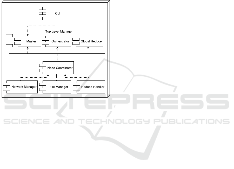
OSGi Bundle, plays a speciﬁc role and interacts with

other bundles. Each site, belonging to the network, is

an independent system and has a full instance of the

middleware; this design choice guarantees the possi-

bility for each node to assume all of the roles. Indeed

the Bottom-Level logic is owned by any site of the

network, but only one node at a time can take the role

of the Top-Level Manager (by enabling speciﬁc mod-

ules).

Figure 2: Overall architecture.

A middleware instance has the modular structure

depicted in Figure 2. Each module is designed to ful-

ﬁll speciﬁc functions. The main modules are:

• Network Manager: it supports the communication

of the node with other nodes in the network.

• CLI: it represents the command line interface to

submit a job execution request to the middleware.

• File Manager: it implements the ﬁle system fea-

tures to keep track of middleware ﬁle namespace.

In this module the system load and storage bal-

ance algorithms are deﬁned.

• Hadoop Handler: it is designed to decouple the

middleware layer from the underlying (plain)

Hadoop platform. It provides the capability to in-

teract with the features offered by plain Hadoop.

• Node Coordinator: this module maintains the

node status and implements the orchestrator’s

election algorithm. Any site is potentially eligi-

ble as Coordinator.

The above described modules are common to all

nodes. The middleware also includes optional mod-

ules that are deployed only on sites playing speciﬁc

roles. The optional modules, which enable the Top-

Level Manager role, are:

• Orchestrator: it monitors the distributed contexts

resources and is responsible for the generation of

a Top-level Job Execution Plan (TJEP).

• Master: this role is taken by the site who receives

the top level job execution request. It asks the or-

chestrator for the job execution plan and enforce

it. It receives the ﬁnal result of job processing

from the Global Reducer and forward it to the job

submitter.

• Global Reducer: it collects all the results obtained

from the execution of sub-job concerning a spe-

ciﬁc job and performs the top-level reduction on

those results.

4.1 The Orchestrator Module

The orchestrator module represents the core compo-

nent of the architecture. Its main tasks are basically

the following ones:

• gathering information on the Sites’ overall avail-

able computing capacity and the inter-site band-

width capacity.

• generating the TJEP, which contains directives on

how data have to be re-distributed among Sites

and on the allocation of sub-jobs that have to be

run on those Sites.

Let us analyze in detail the orchestrator function-

alities. As mentioned before, one of the orchestra-

tor’s task is to acquire knowledge about the resources

distributed in the bottom level’s computing context.

Each Site periodically advertises its capacity to the

Orchestrator. Such capacity represents the overall

computing capacity of the Site for MapReduce pur-

poses (overall nominal capacity). Further, we assume

that Sites enforce a computing capacity’s allocation

policy that reserves a given, ﬁxed amount of capacity

to any submitted MapReduce job. Since the amount

of computing capacity potentially allocable to a sin-

gle job (slot capacity) may differ from Site to Site,

Sites are requested to also communicate that amount

along with the overall nominal capacity. The available

inter-site link capacity is instead “sensed” through a

network infrastructure made of SDN-enabled (Kreutz

et al., 2015) switches. Switches are capable of mea-

suring the instant bandwidth used by incoming and

outgoing data ﬂows. The Orchestrator periodically

enquires the switches to retrieve the bandwidth usage

and elaborates statistics on the inter-site bandwidth

usage. The Orchestrator is thus able to build and

maintain a Computing Availability Table that keeps

track of every sites instant and future capacity, aver-

age capacity in time, and other useful historical statis-

tics on the computing capacity parameter. The in-

A Hadoop based Framework to Process Geo-distributed Big Data

181

formation about the inter-sites links is stored into a

Bandwidth Availability Table.

The described monitoring functionality is strictly

related to the generation of the TJEP. All the infor-

mation collected from the bottom level’s computing

context represent the base knowledge needed for the

deﬁnition of a scheduling strategy. Those data, along

with the proﬁle of the job to be executed, constitute

the input of the scheduling strategy performed by the

Scheduler that is located into the orchestrator module.

Section 5 will describe in details the TJEP generation

process.

5 SCHEDULING STRATEGY

In order to compute the TJEP, the Orchestrator will

call on a scheduling strategy that explores the uni-

verse of all feasible execution paths for that speciﬁc

distributed computing context.

If it may appear clear that the sites’ computing ca-

pacity and the inter-site bandwidth affect the overall

path’s completion time, some words have to be spent

on the impact that the type of MapReduce application

may have on that time. We argue that if the scheduling

system is aware of the application behaviour in terms

of the data produced in output with respect to the data

taken in input, it can use this information to take im-

portant decisions. In a geo-distributed context, mov-

ing big amounts of data back and forth among Sites is

a “costly” operation. If the size of the data produced

by a certain application can be known in advance, this

information will help the scheduling system to decide

on which execution path is best for the application.

In (Heintz et al., 2014) the authors introduce the

α expansion/compression factor, that represents the

ratio of the size of the output data of the Map task of

a MapReduce job to the size of its input data. In our

system focus is on the MapReduce process (not just

on the Map phase) that takes place in a Site. Therefore

we are interested in proﬁling applications as a whole.

We then introduce the data Compression factor

app

, which represents the ratio of the output data size

of an application to its input data size:

app

Out putData

app

InputData

app

(1)

The β

app

parameter may be used to calculate the

amount of data that is produced by a MapReduce job

at a Site, traverses the network and reaches the Global

Reducer. Depending on that amount, the data transfer

phase may seriously impact on the overall top-level

job performance. The exact value of β

app

for a sub-

mitted application may not be known a priori. The

work in (Cavallo et al., 2015) discusses how to get a

good estimate for the β

app

We adopt a graph model to represent the job’s

execution path. Basically, a graph node may rep-

resent either a Data Computing Element (site) or a

Data Transport Element (network link). Arcs be-

tween nodes are used to represent the sequence of

nodes in an execution path. A node is the place where

a data ﬂow arrives (input data) and another data ﬂow

is generated (output data). A node representing a

computing element elaborates data, therefore it will

produce an output data ﬂow whose size is different

than that of input; a node representing a data transport

element just transports data, so input and output data

coincide. Nodes are characterized by two parameters:

the β

app

, that is used to estimate the data produced by

a node, and the Throughput, deﬁned as the amount of

data that the node is able to process per time unit. The

app

value for Data Transport Elements is equal to 1,

because there is no data computation occurring in a

data transfer. As for the Data Computing Element,

instead, β

app

strictly depends on the type of applica-

tion to be executed. In the case of Data Transports

Element, the Throughput is equal to the link capacity.

The Throughput of a Data Computing Elements de-

pends again on both the application type and the Site’s

computing capacity. Finally, arcs between nodes are

labeled with a number representing the size of the data

leaving a node and reaching the next node.

The label value of the arc connecting node j − th

to node ( j + 1) −th is given by:

DataSize

j, j+1

= DataSize

j−1, j

× β

(2)

In Figure 3 an example of a graph branch made of two

nodes and a connecting arc is depicted:

Figure 3: Nodes’ data structure.

A generic node j’s execution time is deﬁned as:

DataSize

j−1, j

T hroughput

(3)

An execution path is then modeled as a graph of

nodes. The scheduling system is therefore requested

to search for the best execution path. The hard part of

the scheduling system work is the generation of all the

potential execution paths. The algorithm used to gen-

erate potential execution paths and to select the best

one is described in Listing 1. It is based on the Integer

CLOSER 2016 - 6th International Conference on Cloud Computing and Services Science

182

Partitioning theory(Andrews, 1976); for a deeper de-

scription of the algorithm steps the reader may refer

to (Cavallo et al., 2015).

1 pa r s i n g_ t op ol o gy _f r om _ co nf i g_ f il e

2 ge t_ ma p pe r _b e ta _a n d_ t hr ou g hp u t

3 mi n i mu m T i m e = m a x V a l u e

4 ge ne ra t e_ m ap p er _ co mb i na t io n s

5 fo r e a c h ( ma p p e r _ co m b in a ti o n )

6 generate ex ec u t i on P a t h

7 d e t e ct _ co nf l ic t s_ in _ ex e cu ti o nP a th

8 wh i l e (! co nf l ic t l is t _i s _e m pt y )

9 r e s o l ve _ co nf l ic t _i n_ e xe c ut io n Pa th

10 e v a l u at e _e x ec u ti o nT i m e

11 if ( e x e c u t io n T i me <= m i n i m u mT i m e )

12 bet s t P a t h L is t . add ( e xe c u t io n P a th )

13 mi n _t r a n sf e r s = m a x _ v a l u e

14 fo r e a c h ( ex e c u ti o nP a th _ in _b e st P at h Li st )

15 tran s f e r s = e v a l ua t e_ n um b er _ of _ tr an s fe r s

16 if ( t r a n sf e r s_ n u mb e r <= m i n_ t r a ns f e r s )

17 be t s tP a t h = e x e c u t i o nP a t h

18 re t u r n b e s tP a t h

Listing 1: TJEP pseudocode.

Let us now explain how to compute the execution

time of a speciﬁc execution path in a reference sce-

nario.

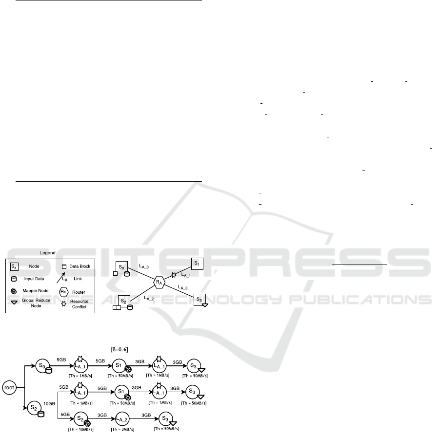
Figure 4: Example scenario topology.

Figure 5: Graph modeling a potential execution path.

Figure 4 depicts a scenario of four sites (S

through S

) and a geographic network interconnect-

ing the sites. A top-level job need to process a 15

GB data set distributed in this way: 5 GB located

in Site S

and 10 GB located in Site S

. Let us as-

sume that one of the execution-paths generated by

the scheduling system involves the movement of 5GB

data from S

to S

, and that three MapReduce sub-

jobs will be executed at S

and S

respectively. The

Global reducing of the data produced by the MapRe-

duce sub-jobs will be performed at S3. In Figure 5

the graph that models a potential execution path for

the just discussed conﬁguration is represented. Basi-

cally, a graph has as many branches as the number of

bottom-level MapReduce (three, in our case). Every

branch starts at the root node (initial node) and ends at

the Global reducer’s node. In the example, the branch

in the bottom models the elaboration of data initially

residing in node S

, that are map-reduced by node S

itself, and results are ﬁnally pushed to node S

(the

Global reducer) through the links L

A 2

and L

A 3

. In the

graph, only the L

A 2

link is represented as it is slower

than L

and will impose its speed in the overall path

→ L

A 2

→ R

→ L

A 3

→ S

. Similarly, in the top-

most branch the data residing in node S

are moved to

node S

through link L

A 1

, are map-reduced by node

and results are pushed to node S

through link L

A 1

In the central branch the data residing in node S

are

moved to node S

through link L

A 1

, are map-reduced

by node S

and results are pushed to node S

through

link L

A 1

. Both the nodes S

and S

try to access the

link L

A 1

. The detected conﬂict on the link L

A 1

must

be resolved before the graph evaluation. Conﬂict res-

olution algorithm is described in detail in section 5.1.

The execution time of a branch is computed as the

sum of the execution times of all the branch’s nodes:

branch

N−1

∑

j=1

DataSize

j, j+1

T hroughput

j+1

(4)

being N the number of nodes in the branch.

The overall execution time estimated for the spe-

ciﬁc execution path is deﬁned as the sum of Global re-

ducer’s execution time and the maximum among the

branches’ execution times:

path

= max

1≤K≤P

(T (K)

branch

) + T hroughput

(5)

The execution time of the Global reducer is given

by the summation of the sizes of the data sets com-

ing from all the branches over the node’s estimated

throughput. This concludes the computation of the

execution time of the considered graph. We remind

that the scheduling system is able to generate many

job’s execution paths, for each of which the execution

time is calculated. In the end, the best path to sched-

ule will be, of course, the one with the shortest time.

5.1 Conﬂicts Detection and Resolution

An execution path is a sequence of steps that termi-

nates with the global reduction of locally elaborated

data. Basically, data blocks traverse inter-site net-

work links that may happen to be shared. Being the

usage of network links not exclusive, the scheduler

must take into account the fact that when two or more

A Hadoop based Framework to Process Geo-distributed Big Data

183

data blocks are traversing the same link, its through-

put is shared among them and, therefore, in that case

the performance offered by the resource “link” to each

traversing data block is not the nominal link through-

put. That said, for each execution path the scheduler

will have to search for any data blocks conﬂicting on

the use of any network link.

The TJEP generation algorithm has been en-

hanced by adding a new feature to manage network

conﬂicts. The conﬂicts management is a two-phases

process:

• Conﬂict Detection: identifying all nodes that re-

quire simultaneous access to the same physical

network resource.

• Conﬂict Resolution: redistributing throughput

among nodes that compete for resource.

As for the detection phase, the scheduler analyzes ev-

ery generated execution path. For a given path, each

node’s start time and end time are stored on a map

(collection of key - value pair) where:

• the key is the concatenation between the re-

source’s Id and the instant of use;

• the value is an object composed by a counter and a

list. The counter is incremented on every attempt

to write on the entry, and represents the number of

simultaneous access to the resource; the list con-

tains the references to the nodes that try to access

the resource at the same time.

Conﬂicts resolution is performed by dividing the total

throughput of the physical network resource among

nodes that are competing for it. Starting from the in-

formation collected in the resources map, it is possible

to detect the graph nodes competing for the resource.

Every node’s throughput is updated according to the

following policy.

The nominal throughput is equally divided among

the nodes that need to access the resource at the same

time. The node’s throughput is computed as follows:

T h

node

T h

nominal

Con f lictOccurrences

where: T h

node

: Node throughput; T h

nominal

: Nominal

throughput; Con f lictOccurrences: number of con-

ﬂicts on the network resource.

At the end of the conﬂicts resolution phase,

the nodes’ throughput values are updated and the

conﬂicts are marked as solved. Starting from the

conﬂicts-free graph model, the execution time esti-

mate is performed.

6 EXPERIMENT RESULTS

To evaluate the performance and the accuracy of TJEP

scheduling algorithm we set up a testbed made of vir-

tual computing instances, which reproduces a geo-

graphically distributed computing context on a small

scale. In the testbed, a computing node (Site) is rep-

resented by a Virtual Machine (VM) instance. Each

node was conﬁgured with 2GB vRam and a Single

vCore CPU that has a theoretical computing power of

15GFLOPS. The reference scenario includes 5 nodes

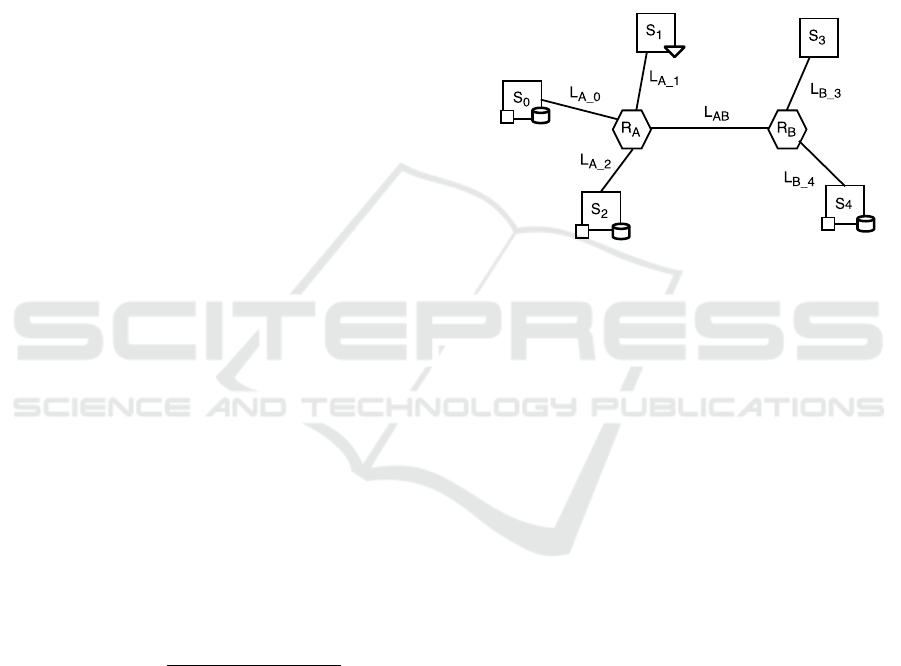
as depicted in Figure 6.

Figure 6: Testbed Topology.

The Sites are connected by a virtualized network

infrastructure. For the test purpose, the links’ capac-

ity was set to 10MB/s each. Experiments were run on

the WordCount application, for which the estimated

compression factors turned out to be β

app

= 0.015.

The datablock size used for our tests was 1 GByte.

When fed with the WordCount conﬁguration, the

scheduler generated 510 potential execution paths in

about less than 3 seconds. The main objective of the

experiment was to compare the performance of the

best execution path generated by our scheduler with

the real job execution time. We run several tests on

the conﬁguration described above. Each test was car-

ried out by modifying the initial data location in order

to analyze the behaviour of the TJEP in different sit-

uations. Table 1 shows the results obtained from the

tests.

As the reader may observe, in all the tests the er-

ror between the TJEP predicted execution time and

the real job execution time was below 10% on aver-

age. The error made by the TJEP is very likely due to

the unpredictability of the performance produced by

the virtual computing environment used to simulate

the geographically distributed environment. Anyway,

the obtained result shows that the TJEP is capable of

making good guess of what to expect in term of per-

formance from the actual computation.

CLOSER 2016 - 6th International Conference on Cloud Computing and Services Science

184

Table 1: Experiment results.

Data block location Global Reducer Real Execution Time [s] Predicted Execution Time [s] Error [%]

753 698 7%

883 812 8%

901 818 9%

998 911 9%

7 CONCLUSION

The gradual increase of the information daily pro-

duced by devices connected to the Internet, com-

bined with the enormous data stores found in tradi-

tional databases, has led to the deﬁnition of the Big

Data concept. MapReduce, and in particular its open

implementation Hadoop, has attracted the interest of

both private and academic research as the program-

ming model that best ﬁt the need for efﬁciently pro-

cess heterogeneous data on a large scale. In this paper

we describe a solution based on hierarchical MapRe-

duce that allows to process big data located in geo-

distributed datasets. Our approach involves the de-

sign and the implementation of a hierarchical Hadoop

framework, considering the available computational

resources, the bandwidth of the links and the simul-

taneous accesses to resources, is able to generate an

execution plan that optimizes the completion time of

a job. A test-bed was implemented to prove the via-

bility of the approach. Future work will focus on the

improvement of the reliability and the accuracy of the

scheduling algorithm.

REFERENCES

Andrews, G. E. (1976). The Theory of Partitions, volume 2

of Encyclopedia of Mathematics and its Applications.

Cavallo, M., Cusm

a, L., Di Modica, G., Polito, C., and

Tomarchio, O. (2015). A scheduling strategy to run

Hadoop jobs on geodistributed data. In CLIOT 2015

- 3rd International Workshop on CLoud for IoT, in

conjunction with the Fourth European Conference

on Service-Oriented and Cloud Computing (ESOCC),

Taormina (Italy).

Dean, J. and Ghemawat, S. (2004). MapReduce: simpliﬁed

data processing on large clusters. In OSDI04: Pro-

ceeding of the 6th Conference on Symposium on op-

erating systems design and implementation. USENIX

Association.

Heintz, B., Chandra, A., Sitaraman, R., and Weissman, J.

(2014). End-to-end Optimization for Geo-Distributed

MapReduce. IEEE Transactions on Cloud Comput-

ing, PP(99):1–1.

Jayalath, C., Stephen, J., and Eugster, P. (2014). From

the Cloud to the Atmosphere: Running MapReduce

across Data Centers. IEEE Transactions on Comput-

ers, 63(1):74–87.

Kim, S., Won, J., Han, H., Eom, H., and Yeom, H. Y.

(2011). Improving Hadoop Performance in Intercloud

Environments. SIGMETRICS Perform. Eval. Rev.,

39(3):107–109.

Kreutz, D., Ramos, F., Esteves Verissimo, P., Es-

teve Rothenberg, C., Azodolmolky, S., and Uhlig, S.

(2015). Software-Deﬁned Networking: A Compre-

hensive Survey. Proceedings of the IEEE, 103(1):14–

76.

Luo, Y., Guo, Z., Sun, Y., Plale, B., Qiu, J., and Li, W. W.

(2011). A Hierarchical Framework for Cross-domain

MapReduce Execution. In Proceedings of the Second

International Workshop on Emerging Computational

Methods for the Life Sciences, ECMLS ’11, pages 15–

22.

Mattess, M., Calheiros, R. N., and Buyya, R. (2013). Scal-

ing MapReduce Applications Across Hybrid Clouds

to Meet Soft Deadlines. In Proceedings of the 2013

IEEE 27th International Conference on Advanced In-

formation Networking and Applications, AINA ’13,

pages 629–636.

OSGi Alliance (2013). Open Service Gateway initiative

(OSGi). Available at http://www.osgi.org/.

Petri, I., Montes, J. D., Zou, M., Rana, O. F., Beach, T.,

Li, H., and Rezgui, Y. (2014). In-transit data analysis

and distribution in a multi-cloud environment using

cometcloud. In International Conference on Future

Internet of Things and Cloud, FiCloud 2014, pages

471–476.

Wright, P. and Manieri, A. (2014). Internet of things in the

cloud - theory and practice. In CLOSER 2014 - Pro-

ceedings of the 4th International Conference on Cloud

Computing and Services Science, pages 164–169.

A Hadoop based Framework to Process Geo-distributed Big Data

185