
Document Clustering Games
Rocco Tripodi
1,2
and Marcello Pelillo
1,2
1
ECLT, Ca’ Focsari University, Ca’ Munich, Venice, Italy
2
DAIS, Ca’ Foscari University, Via Torino, Venice, Italy
Keywords:
Document Clustering, Dominant Set, Game Theory.
Abstract:
In this article we propose a new model for document clustering, based on game theoretic principles. Each doc-
ument to be clustered is represented as a player, in the game theoretic sense, and each cluster as a strategy that
the players have to choose in order to maximize their payoff. The geometry of the data is modeled as a graph,
which encodes the pairwise similarity among each document and the games are played among similar players.
In each game the players update their strategies, according to what strategy has been effective in previous
games. The Dominant Set clustering algorithm is used to find the prototypical elements of each cluster. This
information is used in order to divide the players in two disjoint sets, one collecting labeled players, which
always play a definite strategy and the other one collecting unlabeled players, which update their strategy at
each iteration of the games. The evaluation of the system was conducted on 13 document datasets and shows
that the proposed method performs well compared to different document clustering algorithms.
1 INTRODUCTION
Document clustering is a particular kind of cluster-
ing which involves textual data. The objects to be
clustered can have different characteristics, varying
in length and content. Popular applications of doc-
ument clustering aims at organizing tweets (Sankara-
narayanan et al., 2009), news (Bharat et al., 2009),
novels (Ardanuy and Sporleder, 2014) and medical
documents (Dhillon, 2001). It is a fundamental task in
text mining, with different applications that span from
document organization to language modeling (Man-
ning et al., 2008).
Clustering algorithms tailored for this task are
based on generative models (Zhong and Ghosh,
2005), graph models (Zhao et al., 2005; Tagarelli and
Karypis, 2013) and matrix factorization techniques
(Xu et al., 2003; Pompili et al., 2014). Generative
models and topic models (Blei et al., 2003) try to
find the underlying distribution that created the set
of data objects. One problem with these approaches
is the conditional-independence assumption, which
does not hold for textual data, since they are intrinsi-
cally relational. A popular graph-based algorithm for
document clustering is CLUTO (Zhao and Karypis,
2004), which uses different criterion functions to par-
tition the graph into a predefined number of clus-
ters. The problem with partitional approaches is that
it is necessary to give as input the number of clus-
ters to extract. The underlying assumption behind
models based on matrix factorization, such as Non-
negative Matrix Factorization (NMF) (Lee and Seung,
1999; Ding et al., 2006) is that words which occur
together are associated with similar clusters. (Ding
et al., 2006) demonstrated the equivalence between
NMF and Probabilistic Latent Semantic Indexing, a
popular technique for document clustering. A general
problem, common to all the approaches described, in-
volves the temporal dimension. In fact, for these ap-
proaches is difficult to deal with datasets which evolve
over time and in many real world applications docu-
ments are streamed continuously.
With our approach we try to overcome this prob-
lem, simulating the presence of some clusters into
a dataset and classifying new instances according to
this information. We also try to deal with situations in
which the number of clusters is not given as input to
our algorithm. The problem of clustering new objects
is defined as a game, in which we have labeled play-
ers (clustered objects), which always play the strat-
egy associated to their cluster and unlabeled players
which try to learn their strategy according to the strat-
egy that their co-players are choosing. In this way the
geometry of the data is modeled as a similarity graph,
whose nodes are players (documents), and the games
are played only between similar players.
Tripodi, R. and Pelillo, M.
Document Clustering Games.
DOI: 10.5220/0005798601090118
In Proceedings of the 5th International Conference on Pattern Recognition Applications and Methods (ICPRAM 2016), pages 109-118
ISBN: 978-989-758-173-1
Copyright
c
2016 by SCITEPRESS – Science and Technology Publications, Lda. All rights reserved
109

2 GAME THEORY
Game theory provides predictive power in interac-
tive decision situations. It was introduced by Von
Neumann and Morgenstern (Von Neumann and Mor-
genstern, 1944) in order to develop a mathematical
framework able to model the essentials of decision
making in interactive situations. In its normal-form
representation, it consists of a finite set of players I =
{1,..,n}, a set of pure strategies for each player S
i
=
{s
1
,..., s
n
}, and a utility function u
i
: S
1
×...×S
n
→ R,
which associates strategies to payoffs. Each player
can adopt a strategy in order to play a game and the
utility function depends on the combination of strate-
gies played at the same time by the players involved
in the game, not just on the strategy chosen by a sin-
gle player. An important assumption in game theory
is that the players are rational and try to maximize the
value of u
i
. Furthermore, in non-cooperative games
the players choose their strategies independently, con-
sidering what the other players can play and try to find
the best strategy profile to employ in a game.
A strategy s
∗
i
is said to be dominant if and only if:
u
i
(s
∗
i
,s
−i
) > u
i
(s
i
,s
−i
),∀s
−i
∈ S
−i
where s
−i
denotes the strategy chosen by the other
player(s).
Nash equilibria represent the key concept of game
theory and can be defined as those strategy profiles
in which each strategy is a best response to the strat-
egy of the co-player and no player has the incentive to
unilaterally deviate from his decision, because there
is no way to do better. The players can also play
mixed strategies, which are probability distributions
over pure strategies. Within this setting, the players
choose a strategy with a certain pre-assigned proba-
bility. A mixed strategy profile can be defined as a
vector x = (x
1
,. .. ,x
m
), where m is the number of pure
strategies and each component x
h
denotes the prob-
ability that the player chooses its hth pure strategy.
Each player has a strategy profile which is defined as
a standard simplex,
∆ =
n
x ∈ R :
m
∑
h=1
x
h
= 1, and x
h
≥ 0 for all h
o
(1)
Each mixed strategy corresponds to a point on the
simplex and its corners correspond to pure strategies.
In a two-player game, a strategy profile can be de-
fined as a pair (p,q) where p ∈ ∆
i
and q ∈ ∆
j
. The
expected payoff for this strategy profile is computed
as:
u
i
(p,q) = p · A
i
q , u
j
(p,q) = q · A
j
p (2)
where A
i
and A
j
are the payoff matrices of player i and
j respectively. The Nash equilibrium is computed in
mixed strategies in the same way of pure strategies. It
is represented by a pair of strategies such that each is
a best response to the other.
Evolutionary game theory was introduced by John
Maynard Smith and George Price (Smith and Price,
1973), overcoming some limitations of traditional
game theory, such as the hyper-rationality imposed
on the players. In fact, in real life situations the play-
ers choose a strategy according to heuristics or so-
cial norms (Szab
´
o and Fath, 2007). It was introduced
in biology to explain the ritualized behaviors which
emerge in animal conflicts (Smith and Price, 1973).
In this context, strategies correspond to pheno-
types (traits or behaviors), payoffs correspond to off-
spring, allowing players with a high actual payoff (ob-
tained thanks to its phenotype) to be more prevalent in
the population. This formulation explains natural se-
lection choices between alternative phenotypes based
on their utility function. This aspect can be linked to
rational choice theory, in which players make a choice
that maximizes its utility, balancing cost against ben-
efits (Okasha and Binmore, 2012).
This intuition introduces an inductive learning
process, in which we have a population of agents
which play games repeatedly with their neighbors.
The players, at each iteration, update their beliefs on
the state of the game and choose their strategy accord-
ing to what has been effective and what has not in pre-
vious games. The strategy space of each player i is de-
fined as a mixed strategy profile x
i
, as defined above.
It lives in the mixed strategy space of the game, which
is given by the Cartesian product:
Θ = ×
i∈I
∆
i
. (3)
The expected payoff of a pure strategy e
h
in a single
game is calculated as in mixed strategies (see Equa-
tion 2). The difference in evolutionary game theory is
that a player can play the games with all other play-
ers, obtaining a final payoff which is the sum of all
the partial payoffs obtained during the single games.
The payoff corresponding to a single strategy can be
computed as:
u
i
(e
h
i
) =
n
∑
j=1
(A
i j
x
j
)
h
(4)
and the average payoff is:
u
i
(x) =
n
∑
j=1
x
T
i
A
i j
x
j
(5)
where n is the number of players with whom the
games are played and A
i j
is the payoff matrix among
player i and j. Another important characteristic of
evolutionary game theory is that the games are played
ICPRAM 2016 - International Conference on Pattern Recognition Applications and Methods
110

repeatedly. In fact, at each iteration a player can up-
date his strategy space according to the payoffs gained
during the games, allowing the player to allocate more
probability on the strategies with high payoff, until an
equilibrium is reached, which means that the strategy
spaces of the players cannot be updated, because it is
not possible to obtain higher payoffs.
The replicator dynamic equation (Taylor and
Jonker, 1978) is used In order to find those states,
which correspond to the Nash equilibria of the
games,:
˙x = [u(e
h
,x) −u(x,x)] ·x
h
∀h ∈ S (6)
This equation allows better than average strategies
(best replies) to grow at each iteration. It can be used
as a tool in dynamical systems to analyze frequency-
dependent selection (Nowak and Sigmund, 2004),
furthermore, the fixed points of equation 6 corre-
sponds to Nash equilibria (Weibull, 1997). We used
the discrete time version of the replicator dynamic
equation for the experiments of this article:
x
h
(t + 1) = x
h
(t)
u(e
h
,x)
u(x,x)
∀h ∈ S (7)
where, at each time step t, the players update their
strategies according to the strategic environment, until
the system converges and the Nash equilibria are met.
In classical evolutionary game theory these dynamics
describe a stochastic evolutionary process in which
the agents adapt their behaviors to the environment.
3 DOMINANT SET CLUSTERING
Dominant set clustering generalizes the notion of
maximal clique from unweighted undirected to edge-
weighted graph (Pavan and Pelillo, 2007; Rota Bul
`
o
and Pelillo, 2013). Essentially, this generalization is
relevant because it enables to extraction of compact
structures from a graph in an efficient way. Further-
more, it has no parameters and can be used on sym-
metric and asymmetric similarity graphs. It offers
measures of clusters cohesiveness and measures of
vertex participation to a cluster. It is able to model
the definition of a cluster, which states that a cluster
should have high internal homogeneity and that there
should be high inhomogeneity between the samples in
the cluster and those outside. (Jain and Dubes, 1988).
To model these notions we can use a graph G,
with no self loop, represented by its corresponding
weighted adjacency matrix A = (a
i j
) and consider a
cluster as a subset of vertices in it, C ⊆ V . The aver-
age weighted degree of node i ∈ C with regard to C is
defined as,
awdeg
C
(i) =
1
|C|
∑
j∈C
a
i j
. (8)
We can also define the average similarity among a ver-
tex i ∈ C and a vertex j 6∈ C as,
φ(i, j) = a
i j
− awdeg
C
(i). (9)
The weight of node i with respect to C can be defined
as,
W
C
(i) =
(
1, if |C| = 1
∑
j∈C\{i}
φ
C\{i}
( j, i)W
C\{i}
( j), otherwise
(10)
and the total degree of C is,
W (C) =
∑
i∈C
W
C
(i). (11)
This measure gives us the relative similarity among
vertex i and the vertices in C\{i}, with respect to
the overall similarity between the vertices in cluster
C\{i}. W
C
(i) gives us the measure of vertex partici-
pation to a cluster, which should be homogeneous for
all i ∈ C. More formally, the conditions which en-
able the dominant set to realize the notion of cluster
described above are:
1. W
C
(i) > 0, for all i ∈ C
2. W
C∪{i}
(i) < 0, for all i 6∈ C
the first refers to the internal homogeneity of the clus-
ter and the second refers to the external inhomogene-
ity.
A way to extract structures from graphs, which re-
flects the two conditions described above, is given by
the following quadratic form:
f (x) = x
T
Ax. (12)
Within this interpretation, the clustering task is inter-
preted as that of finding a vector x, that maximize f .
The vector x is is a probability vector, whose compo-
nents express the participation of nodes in the cluster,
so we have the following program:
maximize f (x)
subject to x ∈ ∆.
(13)
A (local) solution of program 13 corresponds to a
maximally cohesive cluster (Jain and Dubes, 1988).
Furthermore we have,
Theorem 1. If S is a dominant subset of vertices, then
its weighted characteristic vector x
S
is a strict local
solution of program 13 (for the proof see (Pavan and
Pelillo, 2007)).
Document Clustering Games
111

By formulating the problem in this way, the solu-
tion of program 13 can be found using the replicator
dynamic equation,
x(t + 1) = x
(Ax)
x
T
Ax
. (14)
In the dominant set framework, the clusters are ex-
tracted sequentially from the graph and a peel-off
strategy is used to remove the data points belonging
to an determined cluster, until there are no points to
cluster or a certain number of clusters have been ex-
tracted.
4 CLUSTERING GAMES
This section describes how document clustering
games are formulated. The steps undertaken to re-
solve the task are as follows: document representa-
tion, data preparation, graph construction, clustering,
strategy space implementation and clustering games.
These steps are described in separate paragraphs be-
low.
4.1 Document Representation
We used the bag-of-words (BoW) model to represent
the documents in a text collection. With this model
each document is represented as a vector indexed ac-
cording to the vocabulary of the corpus. The vocabu-
lary of the corpus is represented as the set of unique
words, which appear in a text collection. It is con-
structed a D × T matrix C, where D is the number
of documents in the corpus and T the number of el-
ements in the vocabulary of the corpus. This kind
of representation is called document-term matrix, its
rows are indexed by the documents and its columns by
the vocabulary terms. Each cell of the matrix t f (d,t),
indicates the frequency of the term t in document d.
This representation can lead to a high dimensional
space, furthermore, the BoW model does not incorpo-
rate semantic information. These problems can result
in bad representations of the data. For this reason, dif-
ferent approaches to balance the importance of each
feature and to reduce the dimensionality of the fea-
ture space have been proposed. The importance of
a feature can be weighted using the term frequency
- inverse document frequency (tf-idf) method (Man-
ning et al., 2008). This technique takes as input a
document-term matrix C and update it with the fol-
lowing equation,
t f -id f (d,t) = t f (d,t) ·log
D
d f (d,t)
(15)
where d f (d,t) is the number of documents containing
the term t. Then the vectors are normalized so that no
bias can occur because of the length of the documents.
Latent Semantic Analysis (LSA) is used to derive
semantic information. (Landauer et al., 1998) and to
reduce the dimensionality of the data. The semantic
information is obtained projecting the documents into
a semantic space, where the relatedness of two terms
is computed considering the context in which they ap-
pear. This technique uses the Single Value Decompo-
sition (SVD) to create an approximation of the term
by documents matrix or tf-idf matrix. It decomposes
a matrix D in:
D = U ΣV
T
, (16)
where Σ is a diagonal matrix with the same dimen-
sions of D and U and V are two orthogonal matrices.
The dimensions of the feature space is reduced to k,
taking into account the first k of the matrices in Equa-
tion (16).
4.2 Data Preparation
Each document i in a corpus D is represented with
a BoW approach. From this data representation it is
possible to adopt different dimension reductions tech-
niques, such as LSA (see Section 1), to achieve a more
compact representation of the data. The new vectors
will be used to compute the pairwise similarity among
documents and to construct, with this information, the
proximity matrix W. As measure for this task, it was
used the cosine distance,
cosθ
v
i
· v
j
||v
i
||||v
j
||
(17)
where the nominator is the intersection of the words
in the two vectors and ||v|| is the norm of the vectors,
which is calculated as:
q
∑
n
i=1
w
2
i
.
4.3 Graph Construction
The proximity matrix obtained, in the previous step,
can be used to represent the corpus D as a graph G,
whose nodes are the documents in D and whose edges
are weighted according to the similarity information
stored in W . Since, the cosine distance acts as a lin-
ear kernel, considering only similarity between vec-
tors under the same dimension, it is common to use a
kernel function to smooth the data and transform the
proximity matrix W into an affinity matrix S (Shawe-
Taylor and Cristianini, 2004). This operation is also
useful because it allows to transform a set of complex
and nonlinearly separable patterns into patterns lin-
early separable (Haykin and Network, 2004). For this
ICPRAM 2016 - International Conference on Pattern Recognition Applications and Methods
112

task we used the classical Gaussian kernel,
ˆs(i, j) = exp
(
−
s
2
i j
σ
2
)
(18)
where s
i j
is the dissimilarity among pattern i and j
computed with the cosine distance and σ is a is a pos-
itive real number which determines the kernel width,
and affects the decreasing rate of ˆs. This parame-
ter is calculated experimentally, since the nature of
the data and the clustering separability indices of the
clusters is not known (Peterson, 2011). The cluster-
ing process can also be helped using graph Lapla-
cian techniques. In fact, these techniques are able
to decrease the weights of the edges between differ-
ent groups of nodes. We use the normalized graph
Laplacian, in some of our experiments, which is com-
puted as L = D
−1/2
ˆ
SD
−1/2
, where D is the degree
matrix of
ˆ
S. Once we have matrix L we can reduce
the number of nodes in it, so that document games
are played only among high similar nodes, this re-
finement is aimed at modeling the local neighborhood
relationships among nodes and can be done with two
different methods, the ε-neighborhood graph, which
maintains only the edges which have a value higher
than a predetermined threshold, ε; and the k-nearest
neighbor graphs, which orders the edges weights in
decreasing order and maintains only the first k.
The effect of these processes is shown in Figure
1. On the main diagonal of the matrix it is possible
to recognize some blocks which represent the clus-
ters of the dataset. The values of those points is low
in the cosine matrix, since it encodes the proximity
of the points. Then the matrix is transformed into a
similarity matrix by the Gaussian kernel, in fact, the
points on the main diagonal in this representation are
high. In the Laplacian matrix, it is possible to note
that some noise was removed from the matrix, the el-
ements far from the diagonal appear now clearer and
the blocks near the diagonal now are more uniform.
Finally the k-nn matrix remove many nodes from the
representation, giving a clear picture of the clusters.
We used the Laplacian matrix for the experiments
with the dominant set, since this framework requires
that the similarity values among the elements of a
cluster are very close to each other. The k-nn graph
was used to run the clustering games, since this
framework does not need many data to classify the
points of the graph.
4.4 Clustering
The clustering phase was conducted using the Domi-
nant Set algorithm to extract the prototypical elements
Figure 1: Different data representations for a dataset with 5
classes of different sizes.
of each cluster. We have developed different imple-
mentations, giving as input the number of clusters to
extract and also without this information, which is not
common in many clustering approaches. It is possible
to think at this situation as the case in which there are
some labeled points in the data and we want to clas-
sify new points according to this evidence.
4.5 Strategy Space Implementation
In the previous step it has been shown that with the
proposed approach, the Dominant Set clustering does
not cluster all the nodes in the graph but only some
of them. These points are used to supply information
to the nodes which have not been clustered. Within
this formulation, it is possible to adopt evolutionary
dynamics to cluster the unlabeled points
The strategy space of each player can be initial-
ized as follows,
s
i j
=
(
K
−1
, if node i is unlabeled.
1, if node i has label j,
(19)
where K is the number of clusters to extract and K
−1
ensures that the constraints required by a game theo-
retic framework are met (see equation (1).
4.6 Clustering Games
Once the graph that models the pairwise similarity
among the players and the strategy space of the games
has been created, it is possible to describe more in de-
tail how the games are formulated.
It is assumed that each player i ∈ I, which partic-
ipates in the games is a document in the corpus and
that each strategy, s ∈ S
i
is a particular cluster. The
players can choose a determined strategy among the
Document Clustering Games
113

set of strategies, each expressing a certain hypothe-
sis about its membership in a cluster and K being the
total number of clusters available. We consider S
i
as
the mixed strategy for player i as described in Sec-
tion 2. The games are played among two similar doc-
uments, i and j, imposing only pairwise interaction
among them. The payoff matrix Z
i j
is defined as an
identity matrix of rank K. This choice is motivated
by the fact that, here all the players have the same
strategy space, we do not know in advance, what is
the range of classes to which the players can be as-
sociated, excluding the labeled points obtained in the
clustering phase. For this reason we have to assume
that a document can belong to all classes.
In this setting the best choice for two similar play-
ers is to be clustered in the same class, which is ex-
pressed by the entry Z
i j
= 1,i = j, of the identity
matrix. In these kinds of games, called imitation
games, the players try to learn their strategy by osmo-
sis, learning by their co-players. Within this formula-
tion, the payoff function for each player is additively
separable and is computed as described in Section 2.
Specifically, in the case of clustering games there are
labeled and unlabeled players, which, as proposed in
(Erdem and Pelillo, 2012), can be divided in two dis-
joint sets, I
l
and I
u
, denoting labeled and unlabeled
players, respectively. These players can be divided
further, taking into account the strategy that they play
without hesitation. In formal terms, we will have K
disjoint subsets, I
l
= {I
l|1
,..., I
l|K
}, where each sub-
set denotes the players that always play their kth pure
strategy.
The labeled players always play the strategy asso-
ciated to their cluster, because they lay on a corner of
the simplex, which is always a rest point (Hofbauer
and Sigmund, 2003). We can say that the labeled
players do not play the game to maximize their pay-
offs, because they have already a determined strategy.
Only unlabeled players play the games, because they
have to decide their cluster membership (strategy).
A strategy which can be suggested by labeled play-
ers, in fact, they act as bias over the choices of unla-
beled players. We recall that the games, formulated in
these terms, always have a Nash equilibrium in mixed
strategies (Nash, 1951) and that the adaptation of the
players to the proposed strategic environment is a nat-
ural consequence in game dynamics, given the fact
that each player gradually adjusts his choices accord-
ing to what other players do (Sandholm, 2010). Once
the equilibrium is reached, the cluster of each player i,
corresponds to the strategy s
i j
, with the highest prob-
ability.
The payoffs of the games are calculated equations
4 and 5, which in this case, with labeled and unlabeled
players, are defined as,
u
i
(e
k
i
) =
∑
j∈I
u
(L
i j
A
i j
x
j
)
h
+
K
∑
k=1
∑
j∈I
l|k
L
i j
A
i j
(h,k) (20)
and,
u
i
(x) =
∑
j∈I
u
x
T
i
L
i j
A
i j
x
j
+
K
∑
k=1
∑
j∈I
l|k
x
T
i
(L
i j
A
i j
)
k
. (21)
5 EXPERIMENTAL SETUP
We measured the performances of the systems using
the accuracy measure (AC) and the normalized mu-
tual information (NMI). AC is calculated with the fol-
lowing equation,
AC =
∑
n
i=1
δ(α
i
,map(l
i
))
n
(22)
where n denotes the total number of documents in the
test, δ(x,y) equals to 1, if x and y are clustered in the
same class; map(L
i
) maps each cluster label l
i
to the
equivalent label in the benchmark. The best mapping
is computed using the Kuhn-Munkres algorithm (Lo-
vasz, 1986). The NMI measure was introduced by
Strehl and Ghosh (Strehl and Ghosh, 2003) and in-
dicates the level of agreement between the clustering
C provided by the ground truth and the clustering C
0
produced by a clustering algorithm. The mutual infor-
mation (MI) between the two clusterings is computed
with the following equation,
MI(C,C
0
) =
∑
c
i
∈C,c
0
j
∈C
0
p(c
i
,c
0
j
) · log
2
p(c
i
,c
0
j
)
p(c
i
) · p(c
0
j
)
(23)
where p(c
i
) and p(c
0
i
) are the probabilities that a doc-
ument of the corpus belongs to cluster c
i
and c
0
i
, re-
spectively, and p(c
i
,c
0
i
) is the probability that the se-
lected document belongs to c
i
as well as c
0
i
at the same
time. The MI information is then normalized with the
following equation,
NMI(C,C
0
) =
MI(C,C
0
)
max(H(C), H(C
0
))
(24)
where H(C) and H(C
0
) are the entropies of C and C
0
,
respectively, This measure ranges from 0 to 1. When
NMI is 1 the two clustering are identical, when it is
0, the two sets are independent. Each experiment was
run 50 times and is presented with standard deviation
(±).
For the evaluation of our approach, we used the
same datasets used in (Zhong and Ghosh, 2005),
where has been conducted an extensive comparison
ICPRAM 2016 - International Conference on Pattern Recognition Applications and Methods
114
of different document clustering algorithms
1
. The test
set is composed of 13 datasets, whose characteristics
are illustrated in Table 1. The datasets have differ-
ent sizes (n
d
), from 204 documents (tr23) to 8580
(sports). The number of classes (K) is different and
ranges from 3 to 10. Another important character-
istic of the datasets is the number of words (n
w
) in
the vocabulary of each dataset, which ranges from
5832 (tr23) to 41681 (classic) and is conditioned by
the number of documents on the dataset and on the
number of different topics in it. The last two features
which describe the datasets are n
c
and Balance. n
c
represents the average number of documents per class
and Balance is the ratio among the number of docu-
ments in the smallest class and in the largest class.
Table 1: Datasets description.
Data n
d
n
v
K n
c
Balance
NG17-19 2998 15810 3 999 0.998
classic 7094 41681 4 1774 0.323
k1b 2340 21819 6 390 0.043
hitech 2301 10800 6 384 0.192
reviews 4069 18483 5 814 0.098
sports 8580 14870 7 1226 0.036
la1 3204 31472 6 534 0.290
la12 6279 31472 6 1047 0.282
la2 3075 31472 6 513 0.274
tr11 414 6424 9 46 0.046
tr23 204 5831 6 34 0.066
tr41 878 7453 10 88 0.037
tr45 690 8261 10 69 0.088
5.1 Basic Experiments
In this section we tested our approach with the entire
feature space of each dataset. The graphs for our ex-
periments are prepared as described in Section 4.
The results of these experiments are shown in Ta-
ble 2 and Table 3 and will be used as point of compar-
ison for the next experiments. The results do not show
a stable pattern, in fact they range from NMI .27 on
the hitech dataset, to NMI .67 on k1b. The reason of
this incongruence is the representation of the datasets,
which in some cases has no good discriminators for
the described objects.
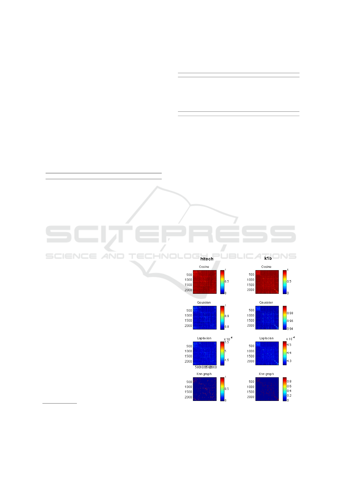
An example of the graphical representation of the
two datasets mentioned above is presented in Fig-
ure 2, where we can see that the similarity matrices
and the corresponding graphs constructed for hitech
do not show a clear structure on the main diagonal.
To the contrary, it is possible to recognize the cluster
structures clearly in the graphs representing k1b.
1
The datasets have been downloaded from,
http://www.shi-zhong.com/software/docdata.zip .
Table 2: Results as AC and NMI, with the entire feature
space.
NG17-19 classic k1b hitech review sports la1
AC .56± 0 .66 ± .07 .82 ± 0 .44 ± 0 .81 ± 0 .69 ± 0 .49 ± .04
NMI .42 ± 0 .56 ± .22 .66 ± 0 .27 ± 0 .59 ± 0 .62 ± 0 .45 ± .04
Table 3: Results as AC and NMI, with the entire feature
space.
la12 la2 tr11 tr23 tr41 tr45
AC .57 ± .02 .54 ± 0 .68 ± .02 .44 ± .01 .64 ± .07 .64 ± .02
NMI .46 ± .01 .46 ± .01 .63 ± .02 .38 ± 0 .53 ± .06 .59 ± .01
5.2 Experiments with Feature Selection
Each dataset described in (Zhong and Ghosh, 2005),
represents a corpus as BoW feature vectors, where
each vector represents a document and each column
indicates the number of occurrences of a particular
word in the corresponding text. This representation
leads to high dimensional space. It gives to each fea-
ture the same importance and does not take into ac-
count the problems of homonymy and synonymy. To
overcome these limitations, we decided to apply to the
corpora a basic frequency selection heuristic, which
eliminates the features which occur more often than
a determined thresholds. In this study only the words
occurring more than once were kept.
This basic reduction leads to a more compact fea-
ture space, which is easier to handle. Words that ap-
Figure 2: Different representations for the datasets hitech
and k1b.
Document Clustering Games
115

Table 4: Number of features for each dataset before and
after feature selection.
classic k1b la1 la12 la2
pre 41681 21819 31472 31472 31472
post 7616 10411 13195 17741 12432
% 0.82 0.52 0.58 0.44 0.6
Table 5: Mean results as AC and NMI, with frequency se-
lection.
classic k1b la1 la12 la2
AC .67 ± 0 .79 ± 0 .56 ± .11 .56 ± .03 .57 ± 0
NMI .57 ± 0 .67 ± 0 .47 ± .12 .44 ± .01 .47 ± 0
pear very few times in the corpus can be special char-
acters or miss-spelled words and for this reason can
be eliminated. The number of features of the new
dataset, after the frequency selection, are shown in Ta-
ble 4. From the table, we can see that the reduction
is significant for five of the datasets used, arriving at
82% of reduction for classic, the other datasets have
not been affected by this process.
In Table 5 we show the results obtained employing
the same algorithm used to test the datasets with all
the features. This reduction can be considered a good
choice to reduce the size of the datasets and the com-
putational, but do not have a big impact on the per-
formances of the algorithm. In fact, the results show
that the improvements, in the performance of the al-
gorithm, are not substantial. We have an improve-
ment of 1%, in terms of NMI, in four datasets over
five. In one dataset we obtained lower results. This
could be due to the fact that we do not know exactly
what words have been removed from the datasets, be-
cause they are not provided with the datasets. In fact,
it is possible that the reduction has removed some im-
portant (discriminative) word from the feature space,
compromising the representation of the documents.
5.3 Experiments with LSA
In this section is presented the evaluation of the pro-
posed approach, using LSA to construct a semantic
space which reduces the dimensions of the feature
space. The evaluation was conducted using different
numbers of features to describe each dataset, ranging
from 10 to 400. This is due to the fact that there is no
agreement on the correct number of features to extract
for a determined dataset. For this reason this value has
to be calculate experimentally.
The results of this evaluation are shown in two dif-
ferent tables, Table 6 indicates the results as NMI and
Table 7 indicates the results as accuracy. The perfor-
mances of the algorithm measured as NMI are sim-
ilar on average (excluding the case of 10 features),
but there is no agreement on different datasets. In
fact, different data representations affect heavily the
performances on datasets such as NG17-19, where
the performances ranges from .27 to .46. This phe-
nomenon is due to the fact that each dataset has dif-
ferent characteristics, as shown in Table 1.
The results with this new representation of the
data shows that the use of LSA is beneficial. In fact,
it is possible to achieve results higher than with the
entire feature space or with the frequency reduction.
The improvements are substantial and in many cases
are 10% higher.
Table 6: Results as NMI for all the datasets. Each column
indicates the results obtained with a reduced version of the
feature space using LSA.
Data 10 50 100 150 200 250 300 350 400
NG17-19 .27 .37 .46 .26 .35 .37 .36 .37 .37
classic .53 .63 .71 .73 .76 .74 .72 .72 .69
k1b .68 .61 .58 .62 .63 .63 .62 .61 .62
hitech .29 .28 .25 .26 .28 .27 .27 .26 .26
reviews .60 .59 .59 .59 .59 .59 .58 .58 .58
sports .62 .63 .69 .67 .66 .66 .66 .64 .62
la1 .49 .53 .58 .58 .58 .57 .59 .57 .59
la12 .48 .52 .52 .52 .53 .56 .54 .55 .54
la2 .53 .56 .58 .58 .58 .58 .59 .58 .58
tr11 .69 .65 .67 .68 .71 .70 .70 .69 .70
tr23 .42 .48 .41 .39 .41 .40 .41 .40 .41
tr41 .65 .75 .72 .69 .71 .74 .76 .69 .75
tr45 .65 .70 .67 .69 .69 .68 .68 .67 .69
avg. .53 .56 .57 .56 .57 .57 .57 .56 .57
Table 7: Results as AC for all the datasets. Each column
indicates the results obtained with a reduced version of the
feature space using LSA.
Data 10 50 100 150 200 250 300 350 400
NG17-19 .61 .63 .56 .57 .51 .51 .51 .51 .51
classic .64 .76 .87 .88 .91 .88 .85 .84 .80
k1b .72 .55 .58 .73 .75 .75 .73 .70 .73
hitech .48 .36 .42 .41 .47 .46 .41 .43 .42
reviews .73 .72 .69 .69 .69 .71 .71 .71 .71
sports .62 .61 .71 .69 .68 .68 .68 .68 .61
la1 .59 .64 .72 .70 .73 .72 .73 .72 .73
la12 .63 .63 .62 .62 .63 .67 .64 .67 .65
la2 .69 .66 .60 .60 .61 .60 .65 .60 .60
tr11 .69 .66 .69 .70 .72 .71 .71 .71 .71
tr23 .44 .51 .43 .42 .43 .43 .43 .43 .43
tr41 .60 .76 .68 .68 .65 .75 .77 .67 .77
tr45 .57 .69 .66 .68 .67 .67 .67 .67 .67
avg. .62 .63 .63 .64 .65 .66 .65 .64 .64
5.4 Evaluation of Document Clustering
Games
The results of the evaluation of the Document Cluster-
ing Games are shown in Table 8 and 9 (third column,
DCG), where, for each dataset, are compared the best
results obtained with the document clustering games
approach and the best results indicated in (Zhong and
Ghosh, 2005) and in (Pompili et al., 2014). In the first
article was conducted an extensive evaluation of dif-
ferent generative and discriminative models, specifi-
ICPRAM 2016 - International Conference on Pattern Recognition Applications and Methods
116

cally tailored for document clustering and two graph-
based approaches, CLUTO and a bipartite spectral
co-clustering method, which obtained better perfor-
mances than the other algorithms. The results in this
article are reported as NMI. In the second article there
is an evaluation on different NMF approaches to doc-
ument clustering, on the same datasets that we used
and the results are reported as AC.
From Table 8 it is possible to see that the results of
the document clustering games are higher than those
of state-of-the-art algorithms on ten datasets out of
thirteen. On the remaining three datasets we obtained
the same results on two datasets and a lower result in
one. On classic, tr23 and tr26 the improvement of our
approach is substantial, with results higher than 5%.
Form Table 9 we can see that our approach performs
substantially better that NMF on all the datasets.
Table 8: Results as NMI of generative models and graph
partitioning algorithm (Best) compared to our approach
with and without the number of clusters to extract.
Data DCG
noK
DCG Best
NG17-19 .39 ± 0 .46 ± 0 .46 ± .01
classic .71 ± 0 .76 ± 0 .71 ± .06
k1b .73 ± .02 .68 ± .02 .67 ± .04
hitech .35 ± .01 .29 ± .02 .33 ± .01
reviews .57 ± .01 .60 ± .01 .56 ± .09
sports .67 ± 0 .69 ± 0 .67 ± .01
la1 .53 ± 0 .59 ± 0 .58 ± .02
la12 .52 ± 0 .56 ± 0 .56 ± .01
la2 .53 ± 0 .59 ± 0 .56 ± .01
tr11 .72 ± 0 .71 ± 0 .68 ± .02
tr23 .57 ± .02 .48 ± .03 .43 ± .02
tr41 .70 ± .01 .76 ± .06 .69 ± .02
tr45 .70 ± .02 .70 ± .03 .68 ± .05
Table 9: Results as AC of NMF models (Best) compared
to our approach with and without the number of clusters to
extract.
Data DCG
noK
DCG Best
NG17-19 .59 ± 0 .63 ± 0 -
classic .80 ± 0 .91 ± 0 .59 ± .07
k1b .86 ± .02 .75 ± .03 .79 ± 0
hitech .52 ± .01 .48 ± .02 .48 ± .04
reviews .64 ± .01 .73 ± .01 .69 ± .07
sports .78 ± 0 .71 ± 0 .50 ± .07
la1 .63 ± 0 .73 ± 0 .66 ± 0
la12 .59 ± 0 .67 ± 0 -
la2 .55 ± 0 .69 ± 0 .53 ± 0
tr11 .74 ± 0 .72 ± 0 .53 ± .05
tr23 .52 ± .02 .51 ± .05 .43 ± .06
tr41 .75 ± .01 .76 ± .08 .53 ± .06
tr45 .71 ± .01 .69 ± .04 .54 ± .06
5.5 Experiments with no Cluster
Number
The last experiment was conducted without using the
number of clusters to extract. It has been tested the
ability of dominant set to find natural clusters and the
performances that can be obtained in this context by
the document clustering games. In this way, we first
run dominant set to discover many small clusters, set-
ting the parameter of the gaussian kernel with a small
value (0.1). Then we re-clusters the obtained clusters
using as similarity matrix the similarities shared be-
tween the nodes of two different clusters.
The results of this evaluation are shown in Table
8 and 9 (second column, DCG
noK
). The results show
that this new formulation of the clustering games per-
forms well in many datasets. In fact, in datasets such
as k1b, hitech, tr11 and tr23 has results higher than
the clustering games performed in the previous sec-
tions. This can be explained by the fact that with this
formulation the number of clustered points is higher
that in the previous version. This can improve the per-
formances of the system when dominant set is able
to find the exact number of natural clusters from the
graph. To the contrary, when it not able to predict
this number, the performances as NMI decrease dras-
tically. This phenomenon can explain why in some
datasets it does not perform well. In fact, in datasets
such as, NG18-19, la1, la12 and l2 the performances
of the system are very low.
6 CONCLUSIONS
In this article we explored new methods for document
clustering based on game theory. We have conducted
an extensive series of experiments to test the approach
on different scenarios. We have also evaluated the
system with different implementations and compared
the results with state-of-the-art algorithms.
Our method can be considered as a continuation
of graph based approaches but it combines together
the partition of the graph and the propagation of the
information across the network. With this method we
used the structural information about the graph and
then we employed evolutionary dynamics to find the
best labeling of the data points. The application of a
game theoretic framework is able to exploit relational
and contextual information and guarantees that the fi-
nal labeling is consistent.
The system has demonstrated to perform well
compared with state-of-the-art system and to be ex-
tremely flexible. In fact, it is possible to implement
Document Clustering Games
117

new graph similarity measure or new dynamics to im-
prove the results or to adapt it to different contexts.
REFERENCES
Ardanuy, M. C. and Sporleder, C. (2014). Structure-based
clustering of novels. EACL 2014, pages 31–39.
Bharat, K., Curtiss, M., and Schmitt, M. (2009). Methods
and apparatus for clustering news content. US Patent
7,568,148.
Blei, D. M., Ng, A. Y., and Jordan, M. I. (2003). La-
tent dirichlet allocation. J. Mach. Learn. Res., 3:993–
1022.
Dhillon, I. S. (2001). Co-clustering documents and words
using bipartite spectral graph partitioning. In Pro-
ceedings of the seventh ACM SIGKDD international
conference on Knowledge discovery and data mining,
pages 269–274. ACM.
Ding, C., Li, T., and Peng, W. (2006). Nonnegative ma-
trix factorization and probabilistic latent semantic in-
dexing: Equivalence chi-square statistic, and a hybrid
method. In Proceedings of the national conference
on artificial intelligence, volume 21, page 342. Menlo
Park, CA; Cambridge, MA; London; AAAI Press;
MIT Press; 1999.
Erdem, A. and Pelillo, M. (2012). Graph transduction
as a noncooperative game. Neural Computation,
24(3):700-723.
Haykin, S. and Network, N. (2004). A comprehensive foun-
dation. Neural Networks, 2(2004).
Hofbauer, J. and Sigmund, K. (2003). Evolutionary game
dynamics. Bulletin of the American Mathematical So-
ciety, 40(4):479–519.
Jain, A. K. and Dubes, R. C. (1988). Algorithms for clus-
tering data. Prentice-Hall, Inc.
Landauer, T. K., Foltz, P. W., and Laham, D. (1998). An in-
troduction to latent semantic analysis. Discourse pro-
cesses, 25(2-3):259–284.
Lee, D. D. and Seung, H. S. (1999). Learning the parts of
objects by non-negative matrix factorization. Nature,
401(6755):788–791.
Lovasz, L. (1986). Matching theory (north-holland mathe-
matics studies).
Manning, C. D., Raghavan, P., Sch
¨
utze, H., et al. (2008).
Introduction to information retrieval, volume 1. Cam-
bridge university press Cambridge.
Nash, J. (1951). Non-cooperative games. Annals of mathe-
matics, pages 286-295.
Nowak, M. A. and Sigmund, K. (2004). Evolutionary dy-
namics of biological games. science, 303(5659):793–
799.
Okasha, S. and Binmore, K. (2012). Evolution and rational-
ity: decisions, co-operation and strategic behaviour.
Cambridge University Press.
Pavan, M. and Pelillo, M. (2007). Dominant sets and pair-
wise clustering. Pattern Analysis and Machine Intel-
ligence, IEEE Transactions on, 29(1):167–172.
Peterson, A. D. (2011). A separability index for clustering
and classification problems with applications to clus-
ter merging and systematic evaluation of clustering al-
gorithms.
Pompili, F., Gillis, N., Absil, P.-A., and Glineur, F. (2014).
Two algorithms for orthogonal nonnegative matrix
factorization with application to clustering. Neuro-
computing, 141:15–25.
Rota Bul
`
o, S. and Pelillo, M. (2013). A game-theoretic
approach to hypergraph clustering. IEEE transac-
tions on pattern analysis and machine intelligence,
35(6):1312–1327.
Sandholm, W. H. (2010). Population games and evolution-
ary dynamics. MIT press.
Sankaranarayanan, J., Samet, H., Teitler, B. E., Lieberman,
M. D., and Sperling, J. (2009). Twitterstand: news
in tweets. In Proceedings of the 17th acm sigspatial
international conference on advances in geographic
information systems, pages 42–51. ACM.
Shawe-Taylor, J. and Cristianini, N. (2004). Kernel methods
for pattern analysis. Cambridge university press.
Smith, J. M. and Price, G. (1973). The logic of animal con-
flict. Nature, 246:15.
Strehl, A. and Ghosh, J. (2003). Cluster ensembles—
a knowledge reuse framework for combining multi-
ple partitions. The Journal of Machine Learning Re-
search, 3:583–617.
Szab
´
o, G. and Fath, G. (2007). Evolutionary games on
graphs. Physics Reports, 446(4):97-216.
Tagarelli, A. and Karypis, G. (2013). Document clustering:
The next frontier. Data Clustering: Algorithms and
Applications, page 305.
Taylor, P. D. and Jonker, L. B. (1978). Evolutionary sta-
ble strategies and game dynamics. Mathematical bio-
sciences, 40(1):145–156.
Von Neumann, J. and Morgenstern, O. (1944). Theory
of Games and Economic Behavior (60th Anniversary
Commemorative Edition). Princeton University Press.
Weibull, J. W. (1997). Evolutionary game theory. MIT
press.
Xu, W., Liu, X., and Gong, Y. (2003). Document clustering
based on non-negative matrix factorization. In Pro-
ceedings of the 26th annual international ACM SI-
GIR conference on Research and development in in-
formaion retrieval, pages 267–273. ACM.
Zhao, Y. and Karypis, G. (2004). Empirical and theoretical
comparisons of selected criterion functions for docu-
ment clustering. Machine Learning, 55(3):311–331.
Zhao, Y., Karypis, G., and Fayyad, U. (2005). Hierarchi-
cal clustering algorithms for document datasets. Data
mining and knowledge discovery, 10(2):141–168.
Zhong, S. and Ghosh, J. (2005). Generative model-based
document clustering: a comparative study. Knowledge
and Information Systems, 8(3):374–384.
ICPRAM 2016 - International Conference on Pattern Recognition Applications and Methods
118
