
A Unified Real-time Automatic Congestion Identification Model
Considering Weather and Roadway Visibility Conditions
Mohammed Elhenawy, Hesham Rakha and Hao Chen
Virginia Tech Transportation Institute, 3500 Transportation Research Plaza, Blacksburg, VA 24061, U.S.A.
Keywords: Transportation Planning and Traffic Operation, Real-time Automatic Congestion Identification, Mixture of
Linear Regression, ITS.
Abstract: Real-time automatic congestion identification is one of the important routines of intelligent transportation
systems (ITS). Previous efforts usually use traffic state measurements (speed, flow, occupancy) to develop
congestion identification algorithms. However, the impacts of weather conditions to identify congestion have
not been investigated in the existing studies. In this paper, we proposed an algorithm that uses the speed probe
data and the corresponding weather and visibility to build a transferable model. This model can be used on
any road stretch. Our algorithm assumes traffic states can be classified into three regimes: congestion, speed
at capacity and free-flow. Moreover, the speed distribution follows a mixture of three components whose
means are functions in weather and visibility. The mean of each component is defined using a linear regression
using different weather conditions and visibility levels as predictors. We used three data sets from VA, CA
and TX to estimate the model parameters. The fitted model is used to calculate the speed cut-off between
congestion and speed at capacity which minimize either the Bayesian classification error or the false positive
(congestion) rate. The test results demonstrate the proposed method produces promising congestion
identification output by considering weather condition and visibility.
1 INTRODUCTION
Traffic congestion has become one of the modern life
problems in many metropolitan areas. This growing
problem has environmental effects. During
congestion time, cars cannot run efficiently so air
pollution, carbon dioxide (CO2) emissions, and fuel
use increase. In 2007, Americans lost $87.2 billion in
wasted fuel and lost productivity. This waste reached
$115 billion in 2009 (Ibrahim and Hall, 1994).
Congestion increases travel time, for example back in
1993 driving under congested condition causes a
delay of about six-tenths of a minute per kilometre of
travel on expressways and 1.2 minutes delay per
kilometre of travel in arterials(Arnott and Small,
1994). The congestion problem becomes worse as
reported by Texas Transportation Institute where the
number of Americans’ wasted hours in traffic
congestion becomes fivefold between 1982 and 2005
Moreover, congestion has its economic effect where
studies show that congestion slow metropolitan
growth, inhibits agglomeration economies, and shape
economic geographies(Sweet, 2011). Traffic
Congestion could result by an obstruction or lack of
road capacity which is a kind of inefficient use of the
roads. This problem can be relaxed by increasing the
road-building budgets to build more infrastructures.
But adding more road capacity is costly and budget is
limited, and the construction itself takes a long time.
With the continuous increase in traffic volumes,
managing traffic, particularly at times of peak
demand, is a good and inexpensive solution to
congestion. Advanced traffic management systems
(ATMS) use various applications of intelligent
transportation systems (ITS) to manage traffic and
reduce congestion problems. Recently, the
advancement in communication and computers
greatly improve ITS and make it more capable of
identifying and reducing congestion. ITS is an
effective solution to traffic problem where it
improves the dynamic capacity of the road system
without building extra expensive infrastructure
(Jianming et al., 2012). Accurate and real-time traffic
information is the foundation of ITS.
Congestion usually starts from a road bottleneck,
then spills over the neighbour road segments. It takes
time until this congestion disappears. Depending on
the frequency of congestion occurrence, traffic
congestion can be divided into two categories
(Guiyan et al., 2010). The first is recurrent traffic
Elhenawy, M., Rakha, H. and Chen, H.
A Unified Real-time Automatic Congestion Identification Model Considering Weather and Roadway Visibility Conditions.
In Proceedings of the International Conference on Vehicle Technology and Intelligent Transport Systems (VEHITS 2016), pages 39-48
ISBN: 978-989-758-185-4
Copyright
c
2016 by SCITEPRESS – Science and Technology Publications, Lda. All rights reserved
39

congestion, and the second is accidental (non-
recurring) traffic congestion. Recurrent traffic
congestion, which usually results from exceeding the
road capacity, is easier to identify and predict. The
accidental traffic congestion usually results from
traffic incident or severe weather conditions. Traffic
congestion is different at different locations, time
periods, and different weather conditions.
The impact of weather on the freeway traffic
operations is a big concern for roadway management
agencies, however, there is little research done to link
weather and congestion in a quantitative sense. Two
groups at the University of Washington correlated
weather and traffic phenomena using the Traffic Data
Acquisition and Distribution (TDAD) data mine and
the Doppler radar data mine (Dailey, 2006). Their
basic idea is that, moving weather cells can be tracked
and predicted using weather radar then they can find
the correlation between the properties of the weather
cell and observed traffic states. Nookala studied the
traffic congestion caused by weather conditions and
its effect on traffic volume and travel time (Nookala,
2006). He observed an increase in the traffic
congestion at inclement weather conditions due to
drop in the freeway capacity while the traffic demand
does not drop significantly. Chung et al. used traffic
data collected over a 2 year period from July first
2002 to June thirty 2004 at Tokyo Metropolitan
Expressway (MEX) and showed a decrease in free
flow speed and in capacity with increasing amount of
rainfall(Chung et al., 2006). Brilon and Ponzlet used
three years of historical data for 15 freeway sites in
Germany to investigate impacts of several factors
including weather on speed-flow relationships
(Brilon and Ponzlet, 1996). They found that wet
roadway conditions cause different speed reduction at
highways with different lane number. Agarwal et al.
highlighted that the results obtained from studies
outside the United States can’t applied within the
United States due to the different roadway and driver
characteristics. Moreover, the result obtained from
rural freeway segments within the United States may
be different from urban freeway(Agarwal et al.,
2005). Ibrahim and Hall used limited historical data
set and multiple regression analysis to study the
impact of rain and snow on speed (Ibrahim and Hall,
1994). Their results showed that light rain and snow
causes similar reductions in speeds (3%–5%), while
14%–15% and 30%–40% reduction in speed are
caused by heavy rain and heavy snow respectively.
Rakha et al used weather data (precipitation and
visibility) and loop detector data (speed, flow, and
occupancy) obtained from Baltimore, Twin Cities,
and Seattle in the USA to quantify the impact of
inclement weather on traffic stream behavior and key
traffic stream parameters, including free-flow speed,
speed-at-capacity, capacity, and jam density. For
more detailed discussion of the Rakha’s result readers
are referred to (Rakha et al., 2007).
During the last few years, many automatic
congestion identification algorithms are proposed.
ASBIA is an algorithm that uses speed measurements
over short temporal and spatial intervals and
segments, respectively to identify the status of a
segment using t-test(Elhenawy et al., 2013). The
outputs of the algorithm are the status of the roadway
segment (free-flow or congested) and the confidence
level of the test (p-value). Another algorithm uses
vehicle trajectories in intelligent vehicle
infrastructure co-operation system (IVICS)(Jianming
et al., 2012). Then the spatial–temporal trajectories
are considered as an image to extract the propagation
speed of congestion wave and construct congestion
template. Finally correlation is evaluated between the
template and the spatial–temporal velocity image to
identify the congestion. Parallel SVM is used in (Sun
et al., 2012) to identify traffic congestion. The authors
propose Parallel SVM instead of SVM because the
training computation cost of SVM is expensive and
congestion identification is a real-time task.
Floating car data is used in (Xu et al., 2013) to find
meaningful congestion patterns. The analysis of the
floating car data is done using a method based on data
cube and the spatial-temporal related relationship of
the slow-speed road segment to identify the traffic
congestion. The research team at the Center for
Sustainable Mobility (CSM) at the Virginia Tech
Transportation institute (VTTI) developed an
algorithm to identify congested segments using a
spatiotemporal speed matrix (Elhenawy and Rakha,
2013). The proposed algorithm fits two log-normal
(or normal) distributions to the training dataset.
To the best of our knowledge, no research
addresses the impacts of both visibility and weather
conditions on congestion identification. In this paper,
the impacts of weather conditions and visibility levels
on the congestion identification algorithm are
investigated by modelling the speed distribution as
mixture of three log-normal components whose
means are linear function of weather condition and
visibility level. So that based on these factors the
three log-normal components may get close or apart
and the cut-off speed is changed. The proposed
algorithm is built using three different data set from
three different states (VA, TX and CA). The results
of our proposed model are promising and reasonable
where, for example, the cut-off speed increases as the
visibility level increases.
VEHITS 2016 - International Conference on Vehicle Technology and Intelligent Transport Systems
40

The remainder of this paper is organized as
follows. First, a brief background of the method used
in this work is given. After that, the proposed
algorithm is introduced. The data sets used in the case
study is described. Subsequently the result of the
experimental work is explained and an illustrative
example is given to show how to implement the
proposed model. Finally, conclusions and
recommendations for future work are presented.
2 MIXTURE OF LINEAR
REGRESSIONS
Finite mixture models are powerful tools in analyzing
a wide variety of random phenomena. They are used
to model random phenomena in many fields
including agriculture, biology, economics, medicine
and genetics. A mixture of linear regressions is one of
the mixture families studied carefully in the literature
(De Veaux, 1989, Faria and Soromenho, 2009). It can
be used to model the speed for different traffic
regimes at different weather condition and visibility
levels.
The mixture of linear regression can be written as:
p
(
y
|
X
)
=
∑
√
e
(1)
Or as
y
=
x
β
+ϵ
withprobabilityλ
x
β
+ϵ
withprobabilityλ
.
.
.
x
β
+ϵ
withprobability1−
∑
λ
(2)
where y
is a response corresponding to a predictors’
vector x
, β
is a vector of regression coefficients for
the j
mixture component, λ
is a mixing probability
of the j
mixture component, ϵ
are normal random
errors, and m is the number of components in mixture
model. Model parameters
ψ={β
,β
,...,β
,σ
,σ
,...,σ
,λ
,λ
,...,λ
}
can be estimated by maximizing the log-likelihood of
Equation (1); given a set of response predictor
pairs(y
,x
),(y
,x
),...,(y
,x
), and using the
Expectation-Maximization algorithm (EM).
2.1 EM Algorithm
The EM algorithm iteratively finds maximum
likelihood estimates by alternating the E-step and M-
step. Let ψ
()
be parameter estimates after the k
iteration. On the E-step, the posterior probability of
the i
observation comes from component j and is
computed as shown in Equation (3).
w
()
=
()
y
x
,ψ
()
∑
()
y
x
,ψ
()
(3)
where ϕ
y
x
,ψ
()
is the probability density
function of the j
component
On the M-step, new parameter estimates ψ
()
maximizing the log-likelihood function in Equation
(1) are calculated, as shown in Equations (4-5).
λ
()
=
∑
()
(4)
β
()
=(X
W
X)
X
W
Y (5)
where X is an nx(p+1) predictor matrix, Y is the
corresponding nx1 response vector, and W is an nxn
diagonal matrix having w
()
along its diagonal
σ
()
=
∑
()
(
()
)
∑
()
(6)
The E-step and M-step are alternated repeatedly
until the incomplete log-likelihood change is
arbitrarily small, as shown in Equation (7).
∏∑
λ
()
ϕ
y
x
,ψ
()
−
∏∑
λ
()
ϕ
y
x
,ψ
()
< (7)
where ξ is a small number
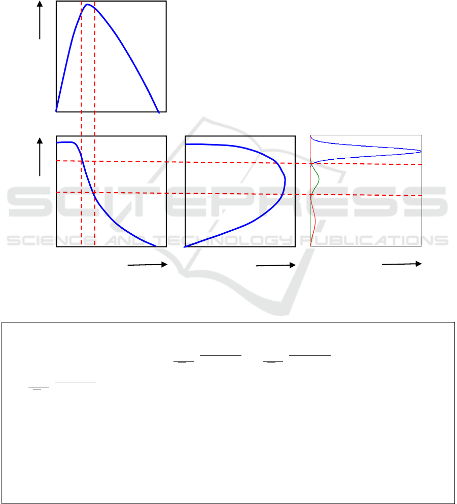
3 PROPOSED ALGORITHM
As shown in the following fundamental diagrams, we
divide the traffic states of a road segment into three
traffic regimes where the speed of each regime can be
modeled by a log-normal distribution. So that the
overall speed distribution can be represented as a
mixture of three log-normal components· First
regime is the free flow which has the speed
distribution with the highest mean. At free flow
regime, the density lies below the capacity density.
The second regime is the Congested flow which has
the speed distribution with the lowest mean. The
congested flow is characterized by the traffic that has
density lies between the capacity density and the jam
density. The third regime is the capacity flow which
separates the free flow from the congested flow and
its speed distribution has a mean that between the
means of the other two regimes. As shown in several
studies the flow fundamental diagram is affected by
the weather conditions (Meead Saberi and Bertini,
A Unified Real-time Automatic Congestion Identification Model Considering Weather and Roadway Visibility Conditions
41
Smith et al., 2003, Rakha et al., 2007). So that we
expect the mean of the speed distribution
corresponding to each regime changes with weather
and visibility. The proposed algorithm uses the
mixture of three linear regression and real data sets to
learn the means of the distribution as a function of
weather and visibility and find the boundary between
the three regimes. The proposed algorithm is shown
below.
All segments with speeds greater than the
threshold are classified as free-flow segments, and
other segments are classified as congested segments.
The output of the above algorithm is a spatiotemporal
binary matrix with dimensions identical to the
spatiotemporal speed matrix. A ‘1’ in the binary
matrix identifies a segment as congested, and a ‘0’
represents free-flow conditions.
Figure 1: Illustration of Link between the Fundamental Diagrams and the Three Components Mixture.
Table 1: The proposed algorithm.
1. Use the EM algorithm described earlier to fit three component distributions to locally-collected data, as demonstrated
in Equation (8).
(
log(y)
|
λ
,λ
,β
,β
,β
,σ
,σ
,σ
)
=λ
√
e
()
+λ
√
e
()
+(1−λ
−
λ
)
√
e
()
, (8)
Where vector is a vector of weather conditions and visibility predictors.
Here (X
β
,σ
) , (X
β
,σ
), and (X
β
,σ
) are the locations and spreads of the mixture components, and (λ
,λ
) are
the mixture parameters.
2. For unseen data use the weather condition, visibility level, and equations of the means (X
β
,X
β
, and X
β
) to
calculate locations (means) of three components.
3. Calculate the cut-off speed. We have two options to calculate the cut-off speed and we can use either of them.
3.1. Calculate 0.001 quintile of the speed at capacity (the middle distribution).
3.2. Calculate cut-off speed using the Bayesian approach; which finds the intersection point (between congestion
and speed at capacity) that minimizes classification error(Elhenawy et al., 2015).
4. Use cut-off speed as a threshold to classify the state of each road segment.
Flow
Speed
Densit
y
Flow
Congested
S
p
eed at ca
p
acit
y
Free-flow
Frequency
VEHITS 2016 - International Conference on Vehicle Technology and Intelligent Transport Systems
42
4 EXPERIMENTAL WORK
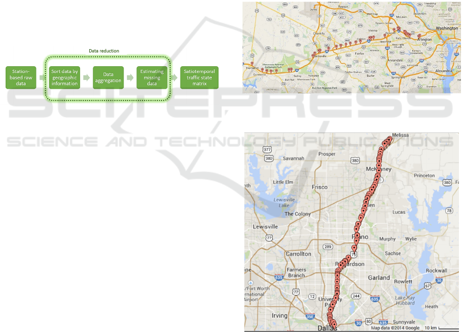
4.1 Data Reduction
In order to use collected traffic data in the proposed
algorithm, data reduction was an important process
for transferring raw measured data into required input
data formats. In general, the spatiotemporal traffic
state matrix is a fundamental attribute of input data.
Reduction of INRIX probe data is one example, and
a similar process can be applied to other types of
measured data (e.g. loop detector). INRIX data are
collected for each roadway segment and time interval.
Each roadway segment represents a TMC station.
Geographic TMC station information is also
provided. The average speed for each TMC station
can be used to derive a spatiotemporal traffic state
matrix. However, raw INRIX data includes
geographically inconsistent sections, irregular time
intervals of data collection, and missing data.
Considering these problems, the data reduction
process is illustrated in Figure 2.
Figure 2: Data Reduction of INRIX Probe Data.
Based on the geographic information of each
TMC station, raw data are sorted along the roadway
direction (e.g. towards eastbound or westbound). An
examination should be adopted to check any
overlapping or inconsistent stations along the
direction. Afterwards, speed data should be
aggregated by time intervals (e.g. 5 minutes),
according to the algorithm’s resolution requirement.
In this way, raw data can be aggregated into a daily
matrix format, along spatial and temporal intervals. It
should be noted that missing data usually exist on the
developed data matrix. Therefore, data imputation
methods should be conducted, to estimate the missing
data by neighbouring cell values. Consequently, the
daily spatiotemporal traffic state matrix can be
generated for congestion and bottleneck
identification.
4.2 Study Sites
INRIX traffic data in three states (Virginia, Texas and
California) were used to develop the proposed
automatic congestion identification algorithm.
Specifically, the study included 2011~2013 data
along I-66 eastbound, 2012 data along US-75
northbound and 2012 data along I-15 southbound.
The selected freeway corridor on I-66 is presented in
Figure 3, which includes 36 freeway segments along
30.7 miles. Average speeds (or travel times) for each
roadway segment are provided in the raw data, which
were collected every minute. In order to reduce the
stochastic noise and measurement error, raw speed
data were aggregated by five-minute intervals.
Therefore, the traffic speed matrix over spatial
(upstream to downstream) and temporal (from 0:00
AM to 23:55 PM) domains could be obtained for each
day. For the other two locations, daily speed matrices
were obtained using the same procedure. Selected
freeway corridors on US-75 and I-15 are presented in
Figure 4 and Figure 5; including 81 segments across
38 miles, and 30 segments across 15.6 miles,
respectively.
Figure 3: Layout of the Selected Freeway Stretch on I-66.
(Source: Google Maps).
Figure 4: Layout of the Selected Freeway Stretch on US-
75. (Source: Google Maps).
A Unified Real-time Automatic Congestion Identification Model Considering Weather and Roadway Visibility Conditions
43
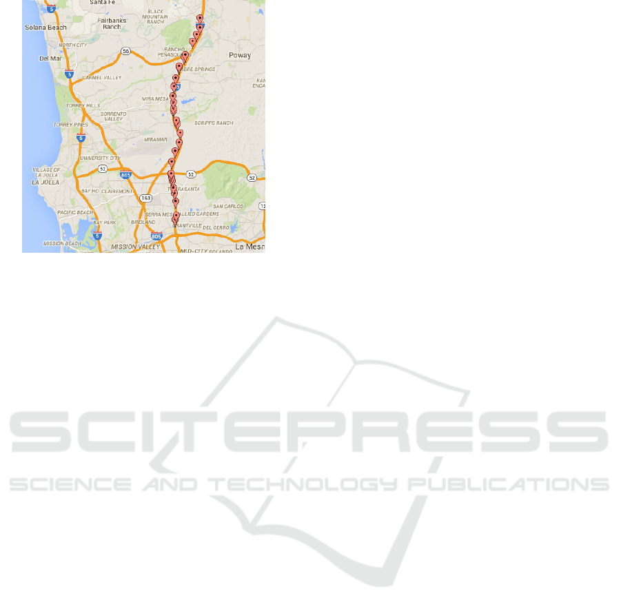
Figure 5: Layout of the Selected Freeway Stretch on I-15.
(Source: Google Maps).
4.3 Effect of Visibility and Weather
Conditions
This subsection describes the investigation of weather
and visibility impacts on the cut-off speed (threshold)
that is used to define the congested condition. The
investigation was limited by the fact that data could
not be divided into bins containing each weather
condition and visibility level. Moreover, many bins
had small amounts of data or no data at all. With this
in mind, the mixture of linear regressions is proposed
to pool data and estimate cut-off speeds, without
sorting the data into clusters. In this subsection, we
describe a speed model, featuring a mix of three linear
regressions. Each linear equation describes a
relationship between independent variables (visibility
and weather) and the dependent variable, which is
speed. In other words, instead of mixing three
components with unchanged means, the speed model
mixed three components whose means were a
function of weather and visibility.
4.4 Unified Model
In order to get a unified model that is independent of
the location or the speed limit, we did the following:
1. Weather conditions for the three data sets
were consolidated based on precipitation.
Weather conditions from all three data sets
were then mapped into these weather
groups. As shown in appendix A. Weather
conditions from all three data sets were then
mapped into these weather groups.
2. We put all the three datasets in one pool and
did not include indicator variables that show
the ID of the dataset.
3. The speed is normalized by dividing the
speed at each road segment by the posted
maximum speed at this segment.
The unified model has a response which is the
normalized speed come from the three datasets and
the predictors are the indicator variables for the
weather groups and the visibility level.
In applying the mixture of three linear regression
model, speed and visibility data were grouped by
weather. Because the data set is huge and we cannot
estimate the model parameters using the whole data
set at once due to memory issues, a total of 7,000
random sample were then drawn randomly from each
weather group, to construct a realization (dataset).
Each random sample includes the speed and visibility
level, together with indicator variables for the
weather. Because speed distributions are skewed, the
log-normal distribution is preferred to the normal
distribution. Log speed was used as the response
variable. Weather code and visibility were the
explanatory variables (predictors). Coefficients of the
predictors(β
,β
,β
), variance of each component
(σ
,σ
,σ
) and proportions (λ
,λ
,λ
) of each
component were estimated using the above iterative
EM algorithm (Equations 3-6). This procedure was
repeated 300 times by bootstrapping the sample
construction without replacement. Final model
parameters were the mean or median of all model
coefficients. Once the final model was derived, we
can observe the shift of the distribution mean with the
weather condition and visibility level in the three
regimes (free-flow, speed at capacity and congested).
Given any combination of weather and visibility. The
final model computes mean speeds for the three
regimes. Furthermore, using the estimated model’s
parameters, the model computes Bayesian and 0.001
quantile cut-off speeds.
The estimated general model’s parameters are
shown in Table 2. As shown figure 6 the results are
sensible because all weather groups have cut-off
speeds lower or equal to the clear group. Moreover,
the cut-off speed increases as visibility increases. We
should mention that the cut-off speed for clear and
light rain are very close so we can apply the cut-off
speed of the clear condition at the light rain as well.
Appendix B shows the speed matrix and the
corresponding binary matrix after applying the
proposed algorithm.
VEHITS 2016 - International Conference on Vehicle Technology and Intelligent Transport Systems
44
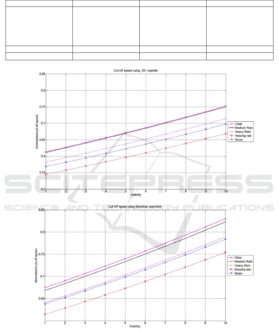
Table 2: Unified model’s parameters.
Congestion Speed at capacity Free flow
'Clear' (Intercept)
'Visibility'
'Medium Rain'
'Heavy Rain'
‘freezing rain’
'Snow'
-0.9025
0.0260
-0.0722
-0.0398
0.2809
0.1754
-0.1947
0.0229
-0.0024
-0.0465
-0.1134
-0.0740
0.0335
0.0026
-0.0238
-0.0308
-0.0018
-0.0149
0.4881 0.1027 0.0680
0.0846 0.1123 0.8028
(a)
(b)
Figure 6: The Unified Model’s Cut-off Speeds (a) Quantile, (b) Bayesian.
4.5 Example Illustration
Recall that, he model that explain the variation in
normalized speed using the weather and visibility is
shown in Equation (9)
A Unified Real-time Automatic Congestion Identification Model Considering Weather and Roadway Visibility Conditions
45

(
log
(
y
)
|
λ
,λ
,β
,β
,β
,σ
,σ
,σ
)
=
λ
√
e
(
)
+λ
√
e
(
)
+
〖(
〗
)
√
e
(
)
,
(9)
Where vector is the vector of weather conditions
and visibility predictors, and y is the normalized
speed. Here (X
β
,σ
) , (X
β
,σ
), and (X
β
,σ
)
are the locations and spreads of the mixture
components and (λ
,λ
) are the mixture parameter.
The above table shows the equations that govern
the locations of the three components are:
=−0.9025+0.0260∗Visibility−
0.0722∗MediumRain−0.0398∗HeavyRain+
0.2809∗freezingrain+0.1754∗Snow
(10)
=−0.1947+0.0229∗
−0.0024∗−0.0465∗
−0.1134∗−
0.0740∗
(11)
=0.0335+0.0026∗−
0.0238∗−0.0308∗−
0.0018∗−0.0149∗ (12)
Let’s give an example to show how to come up
with the Q quantile cut-off speed for given weather
group and visibility level. .Based on the model the
predictors’ vector is as shown in Equation (13)
=
VisibilityMediumRainHeavyRainfreezingrainSnow
(13)
Assume the weather is “” and the
visibility is “2”, what is the Q quantile cut-off speed.
Given the previous information, the predictors’
vector is shown in equation (14),
=
120010
(14)
Then the mean of speed at capacity component is
calculated as shown in equation (15)
=−0.1947+0.0229∗2−0.0024∗
0−0.0465∗0−0.1134∗1−0.0740∗0
(15)
Manipulating the above equation, we get -0.2623 as
the mean of the speed at capacity component. Then
using the Matlab command “norminv(Q, -0.2623,
0.1123)” we get the Q quantile cut-off speed where
0.1123 is the standard deviation for the speed at
capacity component. We should highlights that the
standard deviation and the proportion parameters are
constant and do not depend on the weather group or
visibility.
Now, let assume we are interested in the .001 quantile
at the “” and the visibility is “2”.
Using the Matlab command “norminv(.001, -0.2623,
0.1123)” we get the .001 quantile cut-off speed which
is -0.6093. -0.6093 is the cut-off speed on the log
scale and the cut-off speed used to get the binary
matrix is exp(-0.6093)= 0.5437.In the previous
example, the .001 quantile cut-off speed is 0.5437 of
the posted speed. In other words, the cut-off speed is
0.5437*65= 35.3405 MPH if the posted speed is 65
MPH.
5 CONCLUSIONS
This study developed models of speed distributions in
free-flow, speed at capacity and congested traffic
states using of mixture of linear regressions. To the
best of our knowledge, this is the first methodology
integrates the impact of weather and visibility into
automated congestion identification. Moreover, this
methodology is expected to be more portable because
it is based on three different data set covers three
various regions that hopefully represent the US. The
proposed algorithm is expected to be the state of
practice at many DOTs because of its simplicity,
promising result and suitability to run in real-time
scenarios. Because our algorithm precisely identifies
the traffic congestion, both spatially and temporally,
it is recommended as an important first step towards
identifying and ranking bottlenecks.
ACKNOWLEDGEMENTS
This effort was funded by the Federal Highway
Administration and the Mid-Atlantic University
Transportation Center (MAUTC).
REFERENCES
Agarwal, M., Maze, T. H. & Souleyrette, R. Impacts Of
Weather On Urban Freeway Traffic Flow
Characteristics And Facility Capacity. Proceedings of
the 2005 Mid-Continent Transportation Research
Symposium, 2005.
Arnott, R. & Small, K. 1994. The Economics of Traffic
Congestion. American Scientist, 82, 446-455.
Brilon, W. & Ponzlet, M. 1996. Variability of Speed-Flow
Relationships on German Autobahns. Transportation
Research Record: Journal of The Transportation
Research Board, 1555, 91-98.
VEHITS 2016 - International Conference on Vehicle Technology and Intelligent Transport Systems
46

Chung, E., Ohtani, O., Warita, H., Kuwahara, M. & Morita,
H. Does Weather Affect Highway Capacity. In 5th
International Symposium on Highway Capacity and
Quality of Service, 2006 Yakoma, Japan.
Dailey, D. J. 2006. The Use of Weather Data to Predict
Non-Recurring Traffic Congestion.
De Veaux, R. D. 1989. Mixtures of Linear Regressions.
Computational Statistics & Data Analysis, 8, 227-245.
Elhenawy, M., Chen, H. & Rakha, H. A. Traffic Congestion
Identification Considering Weather and Visibility
Conditions using Mixture Linear Regression. Trans-
portation Research Board 94th Annual Meeting, 2015.
Elhenawy, M. & Rakha, H. 2013. Congestion Identification
with Skewed Component Distributions Vtti.
Elhenawy, M., Rakha, H. A. & Hao, C. An Automated
Statistically-Principled Bottleneck Identification
Algorithm (Asbia). Intelligent Transportation Systems
- (Itsc), 2013 16th International Ieee Conference On, 6-
9 Oct. 2013 2013. 1846-1851.
Faria, S. & Soromenho, G. 2009. Fitting Mixtures Of
Linear Regressions. Journal of Statistical Computation
And Simulation, 80, 201-225.
Guiyan, J., Shifeng, N., Ande, C., Zhiqiang, M. & Chunqin,
Z. The Method Of Traffic Congestion Identification
And Spatial And Temporal Dispersion Range
Estimation. 2nd International Asia Conference On
Informatics In Control, Automation And Robotics
(Car), 2010 6-7 March 2010 2010. 36-39.
Ibrahim, A. T. & Hall, F. L. 1994. Effect Of Adverse
Weather Conditions On Speed-Flow-Occupancy
Relationships.
Jianming, H., Qiang, M., Qi, W., Jiajie, Z. & Yi, Z. 2012.
Traffic Congestion Identification based on Image Pro-
cessing. Intelligent Transport Systems, Iet, 6, 153-160.
Meead Saberi, K. & Bertini, R. L. Empirical Analysis Of
The Effects Of Rain On Measured Freeway Traffic
Parameters.
Nookala, L. S. 2006. Weather Impact on Traffic Conditions
And Travel Time Prediction. Doctoral Dissertation,
University Of Minnesota Duluth.
Rakha, H., Farzaneh, M., Arafeh, M., Hranac, R., Sterzin,
E. & Krechmer, D. 2007. Empirical Studies On Traffic
Flow In Inclement Weather.
Smith, B. L., Byrne, K. G., Copperman, R. B., Hennessy,
S. M. & Goodall, N. J. 2003. An Investigation Into The
Impact Of Rainfall On Freeway Traffic Flow.
Sun, Z.-Q., Feng, J.-Q., Liu, W. & Zhu, X.-M. Traffic
Congestion Identification Based On Parallel Svm.
Natural Computation (Icnc), 2012 Eighth International
Conference On, 29-31 May 2012 2012. 286-289.
Sweet, M. 2011. Does Traffic Congestion Slow The
Economy? Journal of Planning Literature, 26, 391-404.
Xu, L., Yue, Y. & Li, Q. 2013. Identifying Urban Traffic
Congestion Pattern from Historical Floating Car Data.
Procedia - Social and Behavioral Sciences, 96, 2084-
2095.
APPENDIX
Table 3: Six weather groups.
Groups #
Clear 1
Light Rain 2
Rain 3
Heavy rain 4
Freezing rain 5
Snow 6
Figure 7 shows the speed matrix and the corresponding binary matrix after applying the proposed algorithm. The
binary matrix will be further filtered to fill gaps and remove noise using image processing techniques.
A Unified Real-time Automatic Congestion Identification Model Considering Weather and Roadway Visibility Conditions
47
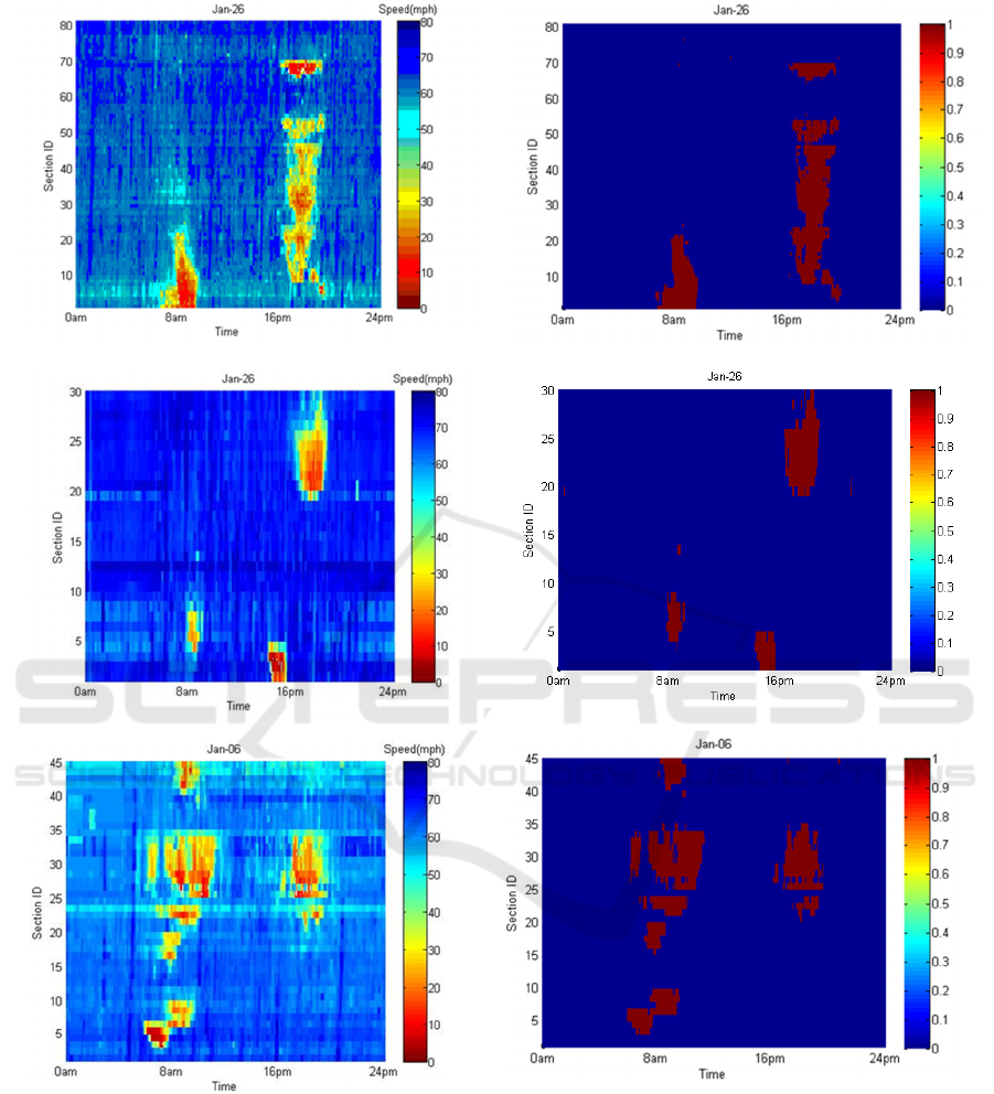
(a)
(b)
(c)
Figure 7: Speed (left) and Binary Matrix after Applying Algorithm (right); (a) TX; (b) CA; (c) VA.
VEHITS 2016 - International Conference on Vehicle Technology and Intelligent Transport Systems
48
