
How Important is Scale in Galaxy Image Classification?
AbdulWahab Kabani and Mahmoud R. El-Sakka
Computer Science Department, The University of Western Ontario, London, Ontario, Canada
Keywords:
Galaxy Classification, Image Classification, Deep Neural Networks, Convolutional Neural Networks,
Machine Learning, Computer Vision, Image Processing, Data Analysis.
Abstract:
In this paper, we study the importance of scale on Galaxy Image Classification. Galaxy Image classification
involves performing Morphological Analysis to determine the shape of the galaxy. Traditionally, Morpholog-
ical Analysis is carried out by trained experts. However, as the number of images of galaxies is increasing,
there’s a desire to come up with a more scalable approach for classification. In this paper, we pre-process the
images to have three different scales. Then, we train the same neural network for small number of epochs
(number of passes over the data) on all of these three scales. After that, we report the performance of the
neural network on each scale. There are two main contributions in this paper. First, we show that scale plays
a major role in the performance of the neural network. Second, we show that normalizing the scale of the
galaxy image produces better results. Such normalization can be extended to any image classification task
with similar characteristics to the galaxy images and where there’s no background clutter.
1 INTRODUCTION
Galaxy classification is a challenging problem. By
studying the shape, color and other properties, scien-
tists can determine the age and acquire information
about the galaxy formation. Such information is vi-
tal in order to understand our universe. Normally, a
trained expert (sometimes even a scientist) is required
to manually classify each image. Such a process does
not scale well, especially given the recent availabil-
ity of large scale surveys such as Sloan Digital Sky
Survey
1
. Recently, The Galaxy Zoo project
2
was
launched in order to classify a large number of im-
ages through on-line crowd sourcing. This classifi-
cation process was very successful as the quality of
the classification was very close to that of an expert.
However, even the Galaxy Zoo project is expected to
not scale well in the near future. This is because tele-
scopes and other imagery devices are able to acquire
images of more distant galaxies. Therefore, it is im-
portant to move away from manual image classifica-
tion into computer based classification.
While the increase in number of galaxy images
makes classical classification methods obsolete, it
presents deep neural networks as a viable option to
classify these images. This is because deep convo-
1
http://www.sdss.org/
2
http://www.galaxyzoo.org/
lutional networks (CNNs) can achieve state-of-the-art
results if there is enough data to train them on. Even
with modest data sizes, they can achieve good results
if a combination of data augmentation and regulariza-
tion is used.
In this paper, we focus on studying the importance
of scale on galaxy image classification. We scale
the images to 64 × 64 and 256 × 256. In addition,
we come up with a normalized scale version of each
galaxy by automatically detecting the scale and crop-
ping the image, accordingly. We test the three ver-
sions of the galaxy image (64 × 64, 256 × 256, and
normalized scale). After that, we resize the images
to 64 × 64 and test them on the same neural network
architecture. We find empirically that the normalized
scale version of the galaxy outperforms the other two
versions. We strongly believe that such findings can
be extended to other image classification problems
with similar characteristics to the galaxy image clas-
sification where there is no background clutter.
This paper is organized as follows: First, we
present a background about deep neural networks in
Section 2. Then, in Section 3, we describe the data
set that we used to do our experiments. Informa-
tion about image pre-processing is found in Section
4. Sections 5, 6, and 7 describe the network architec-
ture, the training process, and implementation details,
respectively. Section 8 presents a set of experiments,
Kabani, A. and El-Sakka, M.
How Important is Scale in Galaxy Image Classification?.
DOI: 10.5220/0005787402630270
In Proceedings of the 11th Joint Conference on Computer Vision, Imaging and Computer Graphics Theory and Applications (VISIGRAPP 2016) - Volume 4: VISAPP, pages 263-270
ISBN: 978-989-758-175-5
Copyright
c
2016 by SCITEPRESS – Science and Technology Publications, Lda. All rights reserved
263

results and some discussion. Finally, we conclude our
work in Section 9.
2 BACKGROUND
Deep learning refers to models that are formed of sev-
eral layers. Such a representation is inspired by the
human vision system where the image is processed
through many different stages in the brain. Each layer
in a neural net consists of several neurons that com-
pute a linear combination of the neurons in the previ-
ous layer. After that, each neuron computes a non-
linear transformation on its weighted combination.
Let X
n−1
, W
n
and b
n
be the input to layer n, a ma-
trix of weights, and a bias, respectively. In addition,
let’s denote the non-linearity by function f . Then,
the output of layer n can be represented as shown in
Equation (1):
X
n
= f (W
n
X
n−1
+ b
n
). (1)
There are many ways to compute non-linearity or
Activation functions f . In the early days, popular
choices included sigmoid functions. Recently, rec-
tified linear units (ReLUs) [ f (x) = max(x, 0)] (Nair
and Hinton, 2010) emerged as an excellent type of
non-linearity for many different problems. Another
popular choice include Parametrized linear unit (Pre-
LUs) (He et al., 2015).
Few years ago, deep neural networks were not
very successful at object classification. This is be-
cause training deep neural networks were very dif-
ficult to train due to a problem known as gradient
vanishing. However, due to advances in comput-
ing power and the introduction of several techniques,
deeper neural networks can be trained.
Proper choice of parameters initialization helps a
lot when training a deep neural network. For example,
pre-training can be used to initialize the values of the
parameters. Another popular option for initialization
include Glorot’s method (Glorot and Bengio, 2010).
Dropout (Srivastava et al., 2014) is an excel-
lent regularization technique, which is essential when
training deep neural networks because it makes sure
that neurons do not co-adapt. It works by randomly
setting some input values from the previous layer to
0. In other words, for each training example, a differ-
ent subset of input values from layer n − 1 is passed
to layer n. This greatly helps in avoiding over-fitting.
Convolutional neural networks (Convnets)
(Fukushima, 1980) is a type of neural network where
the first few layer are called convolutional layers.
The connectivity between convolutional layers is
constrained to produce the behavior of convolution
in digital image processing. Given a stack of feature
maps (or channels), a specific number of filters
(kernels) are learned during training. Convnets were
very successful in the problem of digit recognition,
in which they achieved state of the art results on the
MNIST data set (LeCun et al., 1998). However, they
failed for some time in image object classification.
Thanks to advances in computing power and dif-
ferent techniques such as Dropout (Srivastava et al.,
2014), Glorot’s intitialization method (Glorot and
Bengio, 2010), RelU activations (Nair and Hinton,
2010) and data augmentation, convolutional neural
networks can now handle object recognition prob-
lems.
For example, Convolutional neural networks won
the ImageNet Large scale classification (Deng et al.,
2009; Russakovsky et al., 2015) by a huge margin
(Krizhevsky et al., 2012). Since then, most submis-
sions to the challenge were based on convolutional
neural networks (Szegedy et al., 2014; Simonyan and
Zisserman, 2014).
Convolutional neural networks also achieved ex-
cellent results on the galaxy image classification chal-
lenge. Dieleman et al. (Dieleman et al., 2015) pro-
posed a rotation invariant convnet that achieves ex-
cellent results by exploiting rotation invariance. Their
solution is an ensemble of 17 convnets.
3 THE DATASET
The data that we acquired is a subset of the Galaxy
Zoo 2 data set (Abazajian et al., 2009). Kaggle
3
hosts this subset and allows researchers to download
the data. The size of the data set is 61,578 of labelled
data. Figure 2 shows a small subset of the data.
We extracted 10% of the data set and created a
testing test with the ground truth. As a result, the
size of the training data set becomes 55,420 samples,
while the size of the testing set is 6,158 samples.
Initially, the size of the training set is very low. Af-
ter creating the testing set, the size of the data drops
to 55,420. Therefore, we need to augment the data
in order to have sufficient number of training exam-
ples. There are two types of augmentation: real-time
and static. In real-time augmentation, the data is ran-
domly augmented during training. On other hand,
in static augmentation, the data is augmented before
training. We performed real-time data augmentation,
which means that the CPU generates random trans-
formations on each batch of images before sending
3
https://www.kaggle.com/c/galaxy-zoo-the-galaxy-
challenge
VISAPP 2016 - International Conference on Computer Vision Theory and Applications
264
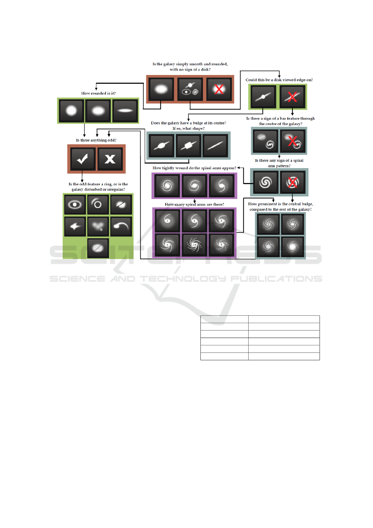
Figure 1: The Galaxy Decision Tree: (Willett et al., 2013). There are 11 questions and 37 answers. During manual classifica-
tion, humans are asked to label each galaxy. Each galaxy labeled multiple times. The classifier has to produce labels that are
as close as possible to the labels produced by humans during the manual labelling process.
them to the GPU for training. This prevents overfit-
ting by ensuring that the GPU receives new training
data batch before calculating each gradient step. Of
course, this is just an illusion as the number of train-
ing images is the same but the training is done on ran-
domly transformed versions of the training images.
The transformations that we have implemented in-
clude a combination of random rotation (angle be-
tween 0 and 360), random horizontal flipping (50%
probability), random vertical flipping (50% probabil-
ity), random horizontal shift (up to 12 pixels), and
random vertical shift (up to 12 pixels). These trans-
formations are summarized in Table 1
The galaxy zoo decision tree (Willett et al., 2013)
(shown in Figure 1) is a tree that consists of 11 ques-
tions with 37 possible answers. This tree determines
the kinds of questions that are asked to participants
during the manual labelling process. Some questions
include “How rounded is the galaxy?”, “Is there any
sign of a spiral arm pattern?”, etc. The task of the
classifier is to predict the 37 possible answers in the
tree.
Table 1: Data Augmentation: Random transformations
along with parameters. These transformations are applied
randomly to each image before sending it to the GPU.
Transformation Parameters
Rotation Angle between 0 and 360
Horizontal Flip randomness=50%
Vertical Flip randomness=50%
Horizontal Shift Up to 12 pixels
Vertical Shift Up to 12 pixels
During the labelling process, the same image is
classified multiple times in order to remove variance
and achieve a classification that is close to that of an
expert. Classifications made by users with good his-
tory of correct labelling are weighted more (Willett
et al., 2013). Our model is expected to predict the 37
probabilities corresponding to the 37 answers in the
tree.
How Important is Scale in Galaxy Image Classification?
265
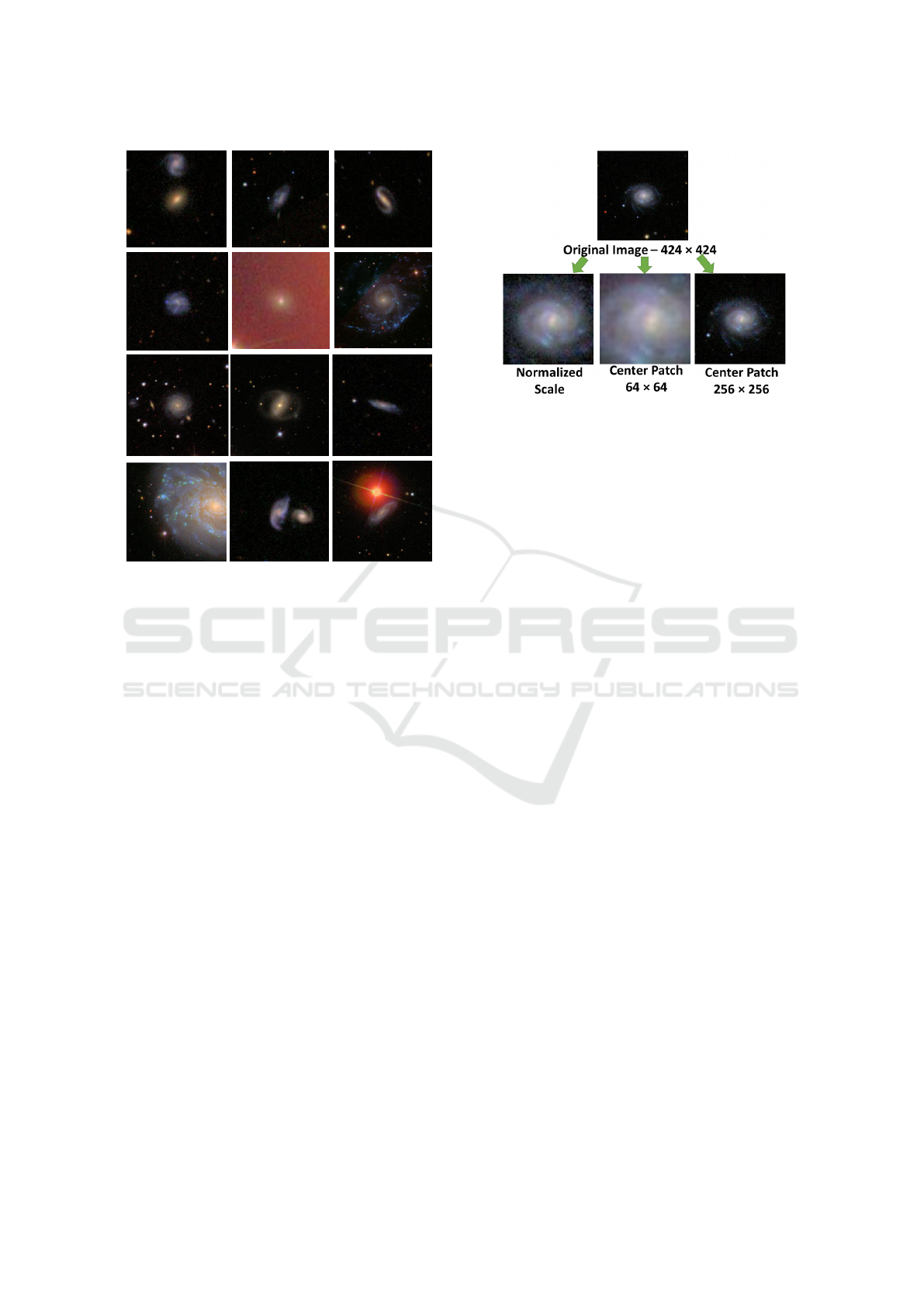
Figure 2: A sample of galaxy images. Most images are
noisy. Some images such as the one in row 2, column 2
is very noisy. Many images contain more than one galaxy
such as the one in row 1, column 1. There is a variety of
objects in the background of many images (for example:
see the image in row 4, column 4).
4 PRE-PROCESSING
The original image size is 424 × 424. Three differ-
ent scale images are extracted from the original im-
age. We trained three neural networks on each type of
scale we extracted. The first scale image is a view of
the galaxy where the scale is normalized such that the
whole galaxy is shown in the image. In order to find
the right scale, the image is first thresholded as shown
in Equation (2),
I(i, j)
thresholded
=
(
1, if I(i, j) ≥ µ
I
+ σ
I
0, otherwise,
(2)
where µ
I
and σ
I
represent the mean and standard
deviation of the image I, respectively.
After that, we find the ellipse that has the same
normalized second central moments as the galaxy
(which is the largest region with pixel value equal to 1
in the center of the image). Finally, the image size is
set to be equal to the major axis length of that ellipse.
For instance, if the major axis length of the ellipse is
120, a patch of size 120 × 120 is extracted from the
center of the image. For the data set we experimented
Figure 3: Three types of images are extracted. Each ex-
tracted image represents a view of the original galaxy at a
specific scale. The amount of cropping for the “normalized
scale” image (left) is determined by cropping the original
image (top) so that the galaxy is filling the whole image.
The second (center) and third (right) images are a result of
extracting the center patch of sizes 64 × 64 and 256 × 256,
respectively. All three images are re-sized (by interpolation)
to have a size of 64 × 64.
with, the galaxy is always located in the center. If
this is not the case, a blob detector such as Laplacian
of Gaussian (LoG) (Bretzner and Lindeberg, 1998) or
Difference of Gaussian (DoG) (Lowe, 2004) can be
used first before finding the ellipse.
The second input image is a result of cropping the
center of the original image to 64 × 64. The third in-
put image was obtained by cropping the center of the
original image to 256 × 256. Finally, the data is stan-
dardized to have the mean equal to zero and standard
deviation equal to one.
5 MODEL ARCHITECTURE
The network accepts an image of size 64 × 64 repre-
senting the galaxy at a specific scale. As mentioned
previously, we train three networks on three types
of images. The first type of input is the normalized
scale image where the galaxy fits perfectly within the
boundary of the image. The second and third type of
input images are the result of cropping the original
image to 64×64 and 256× 256. All input images are
re-sized (by interpolation) to 64 × 64 to ensure that
we have a common ground and architecture to com-
pare the performance of the three neural networks.
As shown in Figure 4, an input image is passed to
the network. After that, it goes through a set of convo-
lutional and pooling layers. Finally, the response goes
through three dense layer (two maxout layers (Good-
fellow et al., 2013) and one linear output layer).
VISAPP 2016 - International Conference on Computer Vision Theory and Applications
266
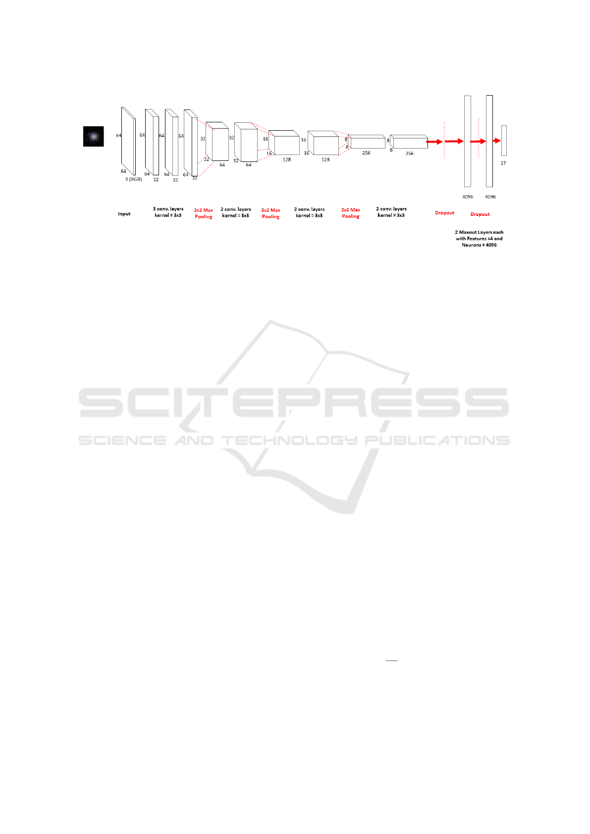
Figure 4: Network Architecture.
We use a relatively small size of convolution ker-
nel. The filters that are used at each layer have a 3 × 3
receptive field with untied biases. In other research
(Simonyan and Zisserman, 2014) and (Szegedy et al.,
2014), it is shown that such a small receptive field
can produce great results if the network is deep
enough. We could not experiment with kernel sizes
such as 11 × 11, and 7 × 7 introduced in other re-
search (Krizhevsky et al., 2012), and (Zeiler and Fer-
gus, 2014), respectively. This is because the size of
the network will grow rapidly and we could not fit it
in the GPU memory we have at our disposal. In addi-
tion, using such a small filter helps us regularize the
network as the number of parameters for the network
becomes very large when using filters with a larger
size. We pad the input image by one pixel across each
dimension to ensure that the spatial resolution does
not decrease after convolution. The nonlinearilty we
used for all convolutional layers is rectified linear unit
(ReLU) (He et al., 2015), (Krizhevsky et al., 2012). A
2 × 2 Max-pooling is carried out three times in the ar-
chitecture. This is important in order to ensure that
the network fits in the GPU. In addition, this allows
the network to learn features even if they are far apart.
As shown in Figure 4, the convolutional segment
consists of (3 convolutional layers and 1 pooling; 2
convolutional layers and 1 pooling; 2 convolutional
layers and 1 pooling; 2 convolutional layers). In total,
the convolutional segment consists of 9 convolutional
layers and 3 pooling layers.
All layers were initialized randomly using the
Glorot initialization (Glorot and Bengio, 2010). We
did not use L1 or L2 regularization rather we relied
solely on dropout (Srivastava et al., 2014), maxout
(Goodfellow et al., 2013), small kernels (Simonyan
and Zisserman, 2014), and data augmentation to reg-
ularize the network.
We use a spatial type of dense layers called max-
out (Goodfellow et al., 2013), which can learn a con-
vex and piecewise linear activation function over the
inputs. Normally, maxout layers are combined with
dropout (Srivastava et al., 2014) to help with train-
ing deep neural networks. We noticed that without
dropout and maxout, training will be difficult due to
overfitting. The dropout rate we used is 50%.
6 TRAINING
As shown in Figure 1, there are 11 classification ques-
tions and 37 answers (the number of leaves in the
decision tree). One neural network is trained to pre-
dict the probability of each of the 37 answers. This is
likely to have a regularization effect on the network as
the weights of the parameters in the network have to
satisfy multiple regression problems. In other words,
we can loosely think of the problem as attempting to
find one solution to satisfy multiple constraints corre-
sponding to the 37 leaves in the decision tree. Despite
the regularizing effect of having one network trained
to solve on multiple regression, the main reason be-
hind having one network is time. Training 37 net-
works to solve this problem may take several months
on a single machine to complete. Obviously, such an
arrangement is not feasible.
During training we need to optimize an objective
functions. Since this is a regression problem, we op-
timize the Mean Square Error (MSE) as it is an excel-
lent choice for solving regression problems. Equation
(3) shows how MSE is computed,
MSE =
1
nm
n
∑
i=1
m
∑
j=1
(
ˆ
Y
i j
−Y
i j
)
2
, (3)
where Y ,
ˆ
Y are true and predicted labels, respectively,
n correspond to the number of training samples, while
m is the number of regression problems (which is 37).
How Important is Scale in Galaxy Image Classification?
267
We use a mini-batch gradient descent (LeCun
et al., 1989) with 0.9 momentum. The batch size was
set to 16 in order to benefit from the randomness in-
troduced by having small batch size. At the begin-
ning, we used a relatively large value for the learn-
ing rate (0.1). After that (at epoch 6), we decreased
this value. We trained the neural network for a to-
tal of 20 epochs (number of passes of the training
data). It is worth noting that much better results can
be achieved by reducing the learning rate to around
(0.05 with a small decay) and training the neural net-
work for around 200 epochs. However, we have not
done that as the main objective of our experiments is
to compare the performance of the net on different
scales rather than optimizing the performance of the
network.
As discussed previously, each image sample goes
through a random transformation as shown in Table
1. This transformation is essential. In fact, we found
that without data augmentation, the network will start
overfitting after around 5 epochs.
7 IMPLEMENTATION
Our implementation relies on Theano (Bastien et al.,
2012), (Bergstra et al., 2010), which is a Python tool-
box for defining, optimizing, and evaluating multi-
dimensional array based mathematical expressions.
In addition, we used Keras
4
, which is a highly mod-
ular neural network library for training on CPUs or
GPUs.
For data pre-prossing and image transformations,
we use scikit-image (van der Walt et al., 2014), which
is a Python library for image processing. The network
is trained in batches. Each batch is transformed on the
CPU and then copied to the GPU for training.
Training each of the neural networks took about
15 hours (for only 20 epochs). Therefore, the total
number of training hours for all three networks is 45
hours. Table 2 shows the specifications of the laptop
we used to carry out the experiments.
Table 2: The technical specifications of the laptop we used
to carry out our experiments.
CPU Intel i7-4710HQ
GPU GTX980M (4 GB)
RAM 24 GB
4
http://www.keras.io/
8 EXPERIMENTS AND
DISCUSSION
In this section, we report the loss functions on each of
the three input types. In addition, we show the non-
deterministic and deterministic scores for each input
type.
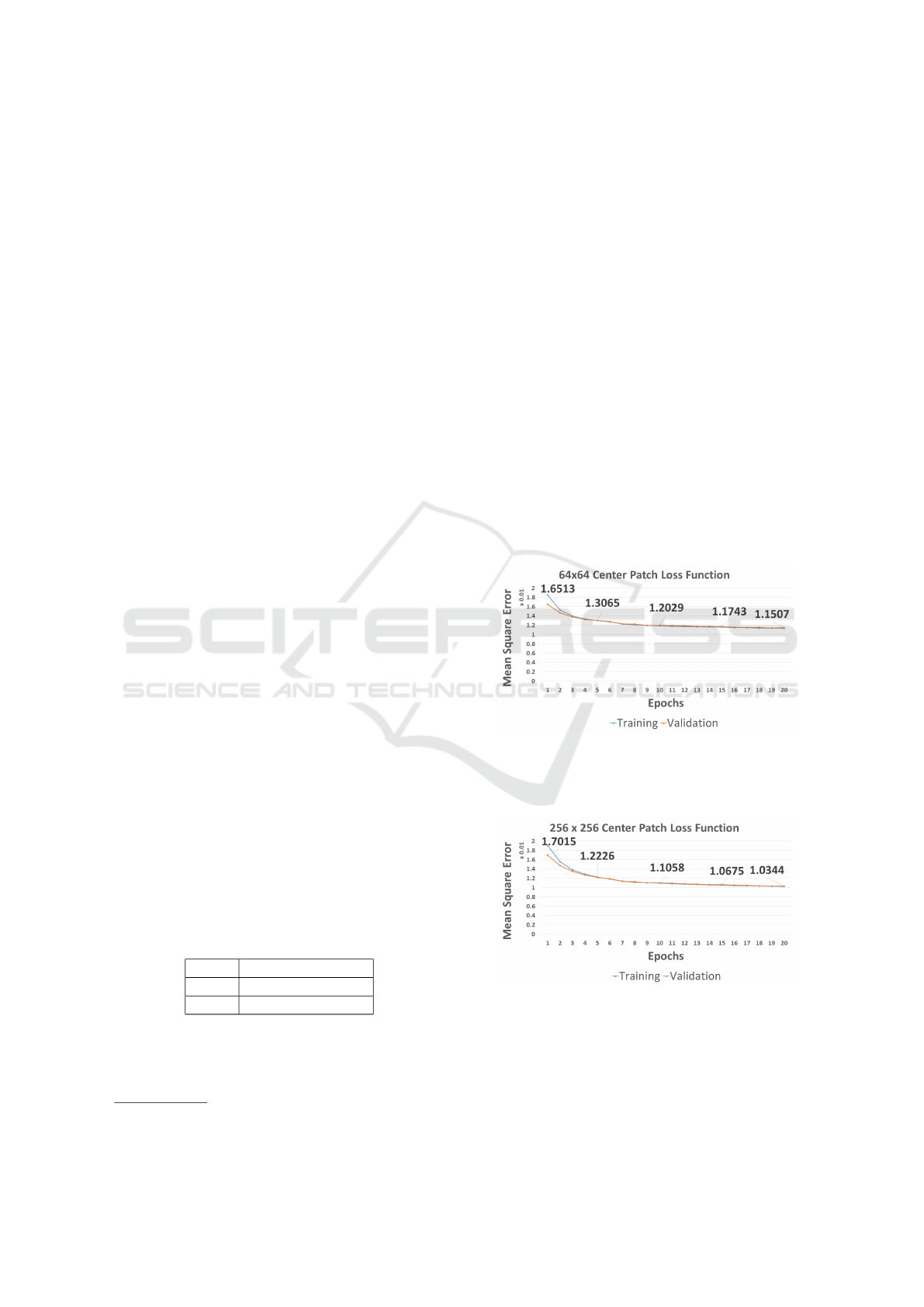
Figures 5 and 6 show the training and validation
losses for input types 64 × 64 and 256 × 256. For in-
put type 64 × 64, the validation loss start from 0.0165
and goes down to 0.0115. On the other hand, as
shown in Figure 6, the validation loss for input type
256×256 starts at a higher loss 0.0170 but goes down
to 0.0103. In other words, although the 256 × 256
loss function starts at a higher value, it outperforms
the loss of the 64 × 64 input after few iterations. In
fact, we found that the 256 × 256 loss is better after
the third epoch. This is likely because the net with
the 256 × 256 input is able to see more information
than the one with input of scale 64 × 64. For exam-
ple, there may be some features around the galaxy that
are helpful for recognition.
Figure 5: 64 × 64 Loss: this Figure shows the loss function
(MSE) during training when the input image has scale of
64 × 64 (A patch of size 64 × 64 was extracted from the
original image).
Figure 6: 256 × 256 Loss: this Figure shows the loss func-
tion (MSE) during training when the input image has a scale
of 256×256 (A patch of size 256 ×256 was extracted from
the original image).
Figure 7, shows the training and validation loss
functions. Here, we can see that the validation loss
starts at a lower (or better) value of 0.0151. This
VISAPP 2016 - International Conference on Computer Vision Theory and Applications
268
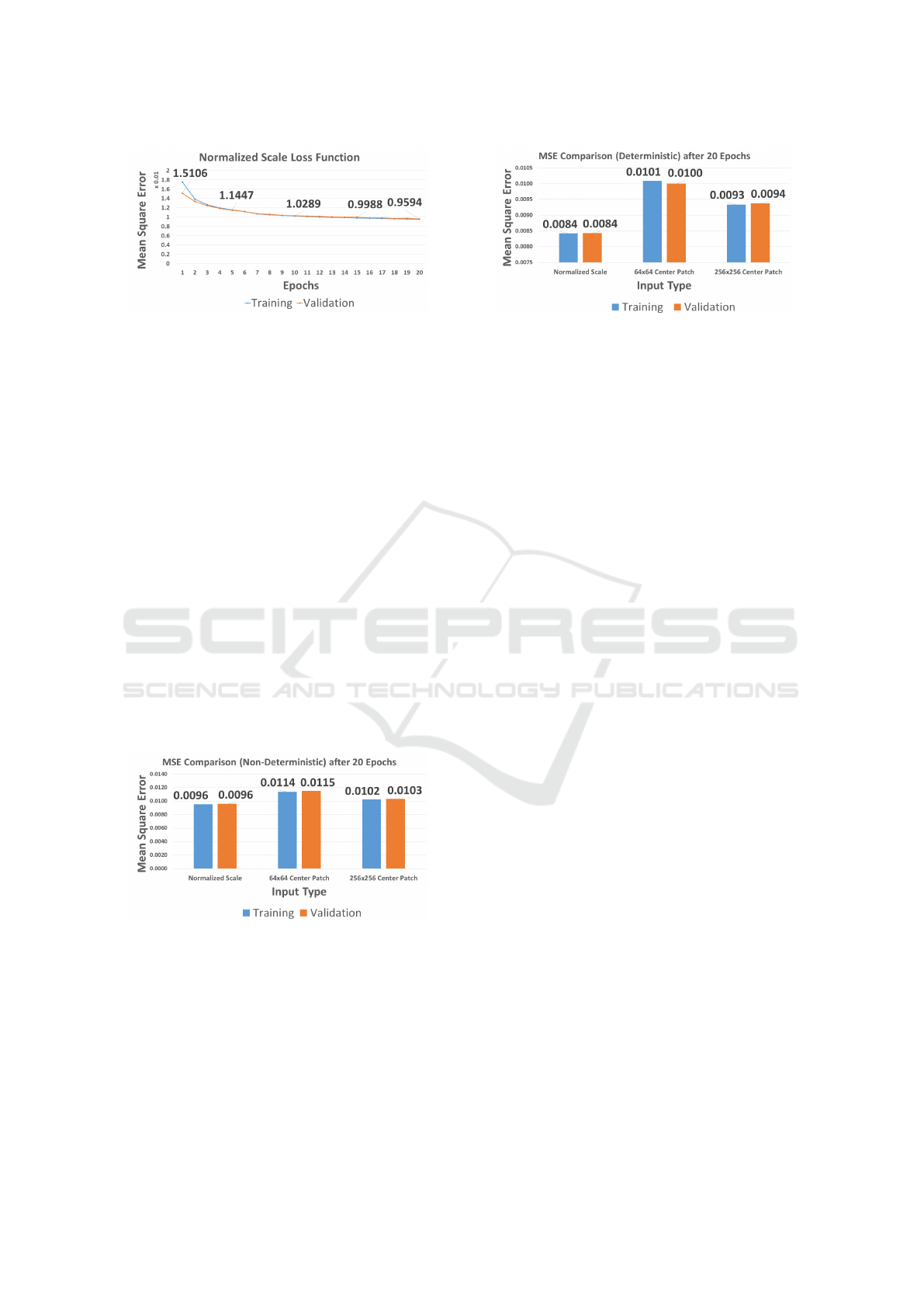
Figure 7: Normalized Scale Loss: this Figure shows the
loss function (MSE) during training when the input image
has normalized scale.
value is much better than the initial loss of both the
64 × 64 and 256 × 256, which starts at 0.0165 and
0.0170, respectively. The normalized scale input also
outperforms the other two input types at the end of
training. At epoch 20, the validation loss for the nor-
malized scale is 0.0095, which is far better than the
other two input types (0.0115 for 64 × 64 and 0.0103
for 256 × 256).
It is worth noting that the training and validation
losses are close to each other. This means that the
net is not overfitting, which is good. It also means
that better performance can be achieved by training
for more epochs and by increasing the size of the net
Figure 8 shows the non-deterministic score (lower
is better) at the end of the training for all input types.
By non-deterministic, we mean that dropout, data
augmentation, and other overfitting prevention tech-
niques are turned on. Again, we can clearly see that
scale normalization achieves excellent results com-
pared to the other two input scales.
Figure 8: Non-deterministic Score: the graph shows the per-
formance after training the neural network for 20 epochs.
By non-deterministic, we mean that the performance is re-
ported with dropout turned on and with data augmentation.
The graph shows the MSE (lower is better). Input with nor-
malized scale outperforms input images scaled by fixed val-
ues 64 × 64 and 256 × 256.
Figure 9 shows the deterministic score where we
turned off dropout, data augmentation, and other over-
fitting prevention techniques. This score is a better
estimation of the production performance. This is be-
Figure 9: Deterministic Score: the graph shows the per-
formance after training the neural network for 20 epochs.
By deterministic, we mean that the performance is reported
with dropout turned off and with data augmentation dis-
abled. In other words, this is the kind of performance one
would expect at production time. The graph shows the MSE
(lower is better). Input with normalized scale outperforms
input images scaled by fixed values 64 × 64 and 256 × 256.
cause overfitting prevention are normally turned off
during testing. We can clearly see that the gap be-
tween the normalized scale input increases. The nor-
malized scale input achieves a score of around 0.0084
as opposed to 0.0100 and 0.0094 for the 64 × 64 and
256 × 256 scales.
Therefore, we conclude that normalizing the scale
of the galaxy image produces better results. This
finding can be easily incorporated into other classi-
fication problems in order to boost the results with a
small time overhead during prepossessing. Scale nor-
malization and cropping of the 61,578 images took
about 20 minutes when performed in parallel (with 4
threads).
It is likely that scale normalization can help with
different classification problems with similar char-
acteristics to the galaxy image classification, where
there is no background clutter and the target object
can be easily distinguished from the background.
9 CONCLUSION AND FUTURE
WORK
We studied the importance of scale in image classifi-
cation that involves training deep convolutional neural
networks. We showed that scale plays a major role in
the performance of the neural network. In addition,
we showed that normalizing the scale of the galaxy
image produces better results. We believe that such
normalization can be extended to any image classifi-
cation task with similar characteristics to the galaxy
images and where there is no background clutter.
In the light of these findings, we plan on incorpo-
rating scale normalization in a slightly larger neural
network we are working to solve the galaxy morpho-
How Important is Scale in Galaxy Image Classification?
269

logical analysis problem. Such model will also incor-
porate the relationships between the predicted labels
values. These relationships are described in the deci-
sion tree in Figure 1. We believe that exploiting these
relationships will likely produce good results.
ACKNOWLEDGEMENTS
This research is partially funded by the Natural Sci-
ences and Engineering Research Council of Canada
(NSERC). This support is greatly appreciated.
REFERENCES
Abazajian, K. N., Adelman-McCarthy, J. K., Ag
¨
ueros,
M. A., Allam, S. S., Prieto, C. A., An, D., Anderson,
K. S., Anderson, S. F., Annis, J., Bahcall, N. A., et al.
(2009). The seventh data release of the sloan digital
sky survey. The Astrophysical Journal Supplement Se-
ries, 182(2):543.
Bastien, F., Lamblin, P., Pascanu, R., Bergstra, J., Good-
fellow, I. J., Bergeron, A., Bouchard, N., and Ben-
gio, Y. (2012). Theano: new features and speed im-
provements. Deep Learning and Unsupervised Fea-
ture Learning NIPS 2012 Workshop.
Bergstra, J., Breuleux, O., Bastien, F., Lamblin, P., Pascanu,
R., Desjardins, G., Turian, J., Warde-Farley, D., and
Bengio, Y. (2010). Theano: a CPU and GPU math
expression compiler. In Proceedings of the Python for
Scientific Computing Conference (SciPy). Oral Pre-
sentation.
Bretzner, L. and Lindeberg, T. (1998). Feature tracking with
automatic selection of spatial scales. Computer Vision
and Image Understanding, 71(3):385–392.
Deng, J., Dong, W., Socher, R., Li, L.-J., Li, K., and Fei-
Fei, L. (2009). ImageNet: A Large-Scale Hierarchical
Image Database. In CVPR09.
Dieleman, S., Willett, K. W., and Dambre, J. (2015).
Rotation-invariant convolutional neural networks for
galaxy morphology prediction. Monthly Notices of the
Royal Astronomical Society, 450(2):1441–1459.
Fukushima, K. (1980). Neocognitron: A self-organizing
neural network model for a mechanism of pattern
recognition unaffected by shift in position. Biologi-
cal cybernetics, 36(4):193–202.
Glorot, X. and Bengio, Y. (2010). Understanding the diffi-
culty of training deep feedforward neural networks. In
International conference on artificial intelligence and
statistics, pages 249–256.
Goodfellow, I. J., Warde-Farley, D., Mirza, M., Courville,
A., and Bengio, Y. (2013). Maxout networks. arXiv
preprint arXiv:1302.4389.
He, K., Zhang, X., Ren, S., and Sun, J. (2015). Delv-
ing deep into rectifiers: Surpassing human-level per-
formance on imagenet classification. arXiv preprint
arXiv:1502.01852.
Krizhevsky, A., Sutskever, I., and Hinton, G. E. (2012). Im-
agenet classification with deep convolutional neural
networks. In Advances in neural information process-
ing systems, pages 1097–1105.
LeCun, Y., Boser, B., Denker, J. S., Henderson, D., Howard,
R. E., Hubbard, W., and Jackel, L. D. (1989). Back-
propagation applied to handwritten zip code recogni-
tion. Neural computation, 1(4):541–551.
LeCun, Y., Bottou, L., Bengio, Y., and Haffner, P. (1998).
Gradient-based learning applied to document recogni-
tion. Proceedings of the IEEE, 86(11):2278–2324.
Lowe, D. G. (2004). Distinctive image features from scale-
invariant keypoints. International journal of computer
vision, 60(2):91–110.
Nair, V. and Hinton, G. E. (2010). Rectified linear units
improve restricted boltzmann machines. In Proceed-
ings of the 27th International Conference on Machine
Learning (ICML-10), pages 807–814.
Russakovsky, O., Deng, J., Su, H., Krause, J., Satheesh, S.,
Ma, S., Huang, Z., Karpathy, A., Khosla, A., Bern-
stein, M., Berg, A. C., and Fei-Fei, L. (2015). Ima-
geNet Large Scale Visual Recognition Challenge. In-
ternational Journal of Computer Vision (IJCV), pages
1–42.
Simonyan, K. and Zisserman, A. (2014). Very deep con-
volutional networks for large-scale image recognition.
arXiv preprint arXiv:1409.1556.
Srivastava, N., Hinton, G., Krizhevsky, A., Sutskever, I.,
and Salakhutdinov, R. (2014). Dropout: A simple way
to prevent neural networks from overfitting. The Jour-
nal of Machine Learning Research, 15(1):1929–1958.
Szegedy, C., Liu, W., Jia, Y., Sermanet, P., Reed, S.,
Anguelov, D., Erhan, D., Vanhoucke, V., and Rabi-
novich, A. (2014). Going deeper with convolutions.
arXiv preprint arXiv:1409.4842.
van der Walt, S., Sch
¨
onberger, J. L., Nunez-Iglesias, J.,
Boulogne, F., Warner, J. D., Yager, N., Gouillart,
E., Yu, T., and the scikit-image contributors (2014).
scikit-image: image processing in Python. PeerJ,
2:e453.
Willett, K. W., Lintott, C. J., Bamford, S. P., Masters, K. L.,
Simmons, B. D., Casteels, K. R., Edmondson, E. M.,
Fortson, L. F., Kaviraj, S., Keel, W. C., et al. (2013).
Galaxy zoo 2: detailed morphological classifications
for 304 122 galaxies from the sloan digital sky survey.
Monthly Notices of the Royal Astronomical Society,
page stt1458.
Zeiler, M. D. and Fergus, R. (2014). Visualizing and un-
derstanding convolutional networks. In Computer
Vision–ECCV 2014, pages 818–833. Springer.
VISAPP 2016 - International Conference on Computer Vision Theory and Applications
270
