
Performance of Interest Point Descriptors
on Hyperspectral Images
Przemysław Głomb and Michał Cholewa
Institute of Theoretical and Applied Informatics, Polish Academy of Sciences,
Bałtycka 5, 44-100 Gliwice, Poland
Keywords:
Hyperspectral Images, Interest Point Descriptors, SIFT, SURF, ORB, BRISK.
Abstract:
Interest point descriptors (e.g. Scale Invariant Feature Transform, SIFT or Speeded-Up Robust Features,
SURF) are often used both for classic image processing tasks (e.g. mosaic generation) or higher level machine
learning tasks (e.g. segmentation or classification). Hyperspectral images are recently gaining popularity as
a potent data source for scene analysis, material identification, anomaly detection or process state estimation.
The structure of hyperspectral images is much more complex than traditional color or monochrome images,
as they comprise of a large number of bands, each corresponding to a narrow range of frequencies. Because
of varying image properties across bands, the application of interest point descriptors to them is not straight-
forward. To the best of our knowledge, there has been, to date, no study of performance of interest point
descriptors on hyperspectral images that simultaneously integrate a number of methods and use a dataset with
significant geometric transformations. Here, we study four popular methods (SIFT, SURF, BRISK, ORB) ap-
plied to complex scene recorded from several viewpoints. We presents experimental results by observing how
well the methods estimate the 3D cameras’ positions, which we propose as a general performance measure.
1 INTRODUCTION
Computer vision applications such as image regis-
tration, stereo matching, object and texture recogni-
tion, image retrieval, robot simultaneous location and
mapping (SLAM) require working with images of
the same scene that were taken at different locations
and times. Changes in geometry, scene composition,
lighting, sensors used to capture images introduce de-
formations in pixel structure that require specialized
algorithms to process. A successful and established
approach for this is to use local features (Mikolajczyk
and Schmid, 2005; Moreels and Perona, 2007): locate
image points with unique characteristics of local pixel
neighbourhood, generate their signature descriptors,
then match those descriptors across different images.
As descriptors are engineered to be robust to potential
degradations (Lowe, 2004; Bay et al., 2008) (affine
transformations, change of geometry,noise, light etc.)
the result should be a match of local areas in two im-
ages with high degree of certainty. This match forms
the base of subsequent processing, which could be de-
tecting the presence of certain objects in images or es-
timating the geometric transformation between them,
e.g. a homography.
Hyperspectral images combine the spatial dimen-
sion of traditional photography with spectral dimen-
sion of spectrographs. The recorded spectral data is
the result of an interaction of light with surfaces of
objects in the scene, thus can be used to identify the
materials much more reliably than RGB information.
Because of the physical properties of this recording
setting, the images from each band (each being es-
sentially a monochromaticbitmap) differin properties
(Mukherjee et al., 2009): amount and characteristics
of noise, level of blur, more or less pronounced fea-
tures (e.g. edges) at given spatial position.
Since their introduction, the local interest point
descriptors have been subject of numerous
1
applica-
tions and comparisons studies. Various techniques
are used for their computation, including Difference
of Gaussians (DoG) filter and image gradients (Lowe,
2004), Haar-like features from integral images (Bay
et al., 2008) or local intensity comparisons (Leuteneg-
ger et al., 2011; Rublee et al., 2011). High dimen-
sional descriptors have been shown to be more ro-
bust to geometric transformations than region corre-
1
As of 2015, the paper introducing one of the most pop-
ular methods (SIFT descriptor) has already over 30K cita-
tions (source: Google Scholar).
200
Głomb, P. and Cholewa, M.
Performance of Interest Point Descriptors on Hyperspectral Images.
DOI: 10.5220/0005785001980203
In Proceedings of the 11th Joint Conference on Computer Vision, Imaging and Computer Graphics Theory and Applications (VISIGRAPP 2016) - Volume 3: VISAPP, pages 200-205
ISBN: 978-989-758-175-5
Copyright
c
2016 by SCITEPRESS – Science and Technology Publications, Lda. All rights reserved

lation (Mikolajczyk and Schmid, 2005). Their per-
formance is consistent across different experimental
settings (Moreels and Perona, 2007). At the same
time, while there have been extensions to multispec-
tral images (see e.g. (Brown and Susstrunk, 2011)),
the studies performed on hyperspectral images have
been comparatively limited. Hyperspectral images
substantially differ from RGB or monochromeimages
because of, among else, much larger data size, vary-
ing performance of sensor of different frequencies,
complex statistical relationships between recorded
spectra, variation in data resulting from push-broom
recording scheme, and varying noise across frequency
spectrum (Mukherjee et al., 2009; Vakalopoulou and
Karantzalos, 2014). While they can be reduced to
monochrome images (that could be a simple input
to classical interest point algorithms), that conver-
sion is not trivial and could lose structural information
(Dorado-Munoz et al., 2012). Most approaches in hy-
perspectral domain are based on the SIFT algorithm:
as classification support (Xu et al., 2008), algorithm
extension (Mukherjee et al., 2009; Dorado-Munoz
et al., 2012), aligning image strips for change detec-
tion (Ringaby et al., 2010) or optimizing parameters
for hyperspectral image matching (Sima and Buckley,
2013). A different approach is taken in (Vakalopoulou
and Karantzalos, 2014), where SIFT and SURF are
combined in working with spectral bands groups.
We identify two important practical shortcom-
ings of current studies. One is the lack of in-
cluding a significant geometric deformations in the
test data set–currently used images differ by time
of acquisition and selected affine parameters only
(translation (Mukherjee et al., 2009; Ringaby et al.,
2010; Dorado-Munoz et al., 2012; Vakalopoulou
and Karantzalos, 2014) and scale (Dorado-Munoz
et al., 2012)), obtained by down-looking satellite or
plane-mounted camera. The only exception is (Sima
and Buckley, 2013), where tripod-acquired geologi-
cal data show some geometric deformations. The sec-
ond problem is the lack of comparing side-by-side the
performance of different methods. The focus is com-
monly on only one method, even at verification stage
(Xu et al., 2008; Mukherjee et al., 2009; Ringaby
et al., 2010; Dorado-Munoz et al., 2012; Sima and
Buckley, 2013). The one exception is (Vakalopoulou
and Karantzalos, 2014), where SIFT and SURF are
compared.
Our focus in this paper is the investigation of
performance of interest point descriptors on hyper-
spectral images of a 3D scene. We make two novel
contributions: first, we compare four separate de-
scriptor algorithms: SIFT (Lowe, 2004), SURF (Bay
et al., 2008), ORB (Rublee et al., 2011) and BRISK
(Leutenegger et al., 2011); second, we use a specially
prepared dataset of scene of mixed natural and man-
made objects, imagined from different view points.
Our experimental setting is as follows: we use the in-
terest point algorithms to detect and match points in
two images, then evaluate them based on quality of
estimation of relative 3D camera positions.
This paper is organized as follows: next section
presents the experimental setting. The results are
presented in the third section, and the last section
presents discussion and concluding remarks.
2 METHODS
Data Set. To compare the descriptors, we use a spe-
cially prepared data set that allows to test image pro-
cessing methods on images with significant geometric
deformations, resulting from hyperspectral imagining
a 3D scene with total viewpoint change of about 45
o2
.
To our best knowledge, this is the first dataset of such
kind.
We use a scene (cf. Figure 1) containing both nat-
ural and artificial fruits of several categories. This
produces images rich in structure in both visual and
NIR spectral ranges (in the former, color based edges
are the strongest, in the latter, neighborhoods of
materials of different types). The scene also con-
tains checkerboard-type markers for calibration and
ground-truth estimation, and Munsell grey panel for
light calibration. The scene is lighted with multi point
halogen light, supported by UV lamp (Omnilux CFL
UV 25W with color temperature 6000 UV K). Images
are recorded with Surface Optics SOC-710VP 375-
1045 nm camera from five points. The angle steps
are at ≈ 11
o
intervals, this choice is based on analy-
sis of (Moreels and Perona, 2007), where it has been
observed that viewpoint change of more than at 30
o
drastically reduces the feature matching effectiveness.
Descriptors. For comparison, we select four de-
scriptors: SIFT (Lowe, 2004) and SURF (Bay et al.,
2008) because of their popularity and reported good
performance; and ORB (Rublee et al., 2011) and
BRISK (Leutenegger et al., 2011), proposed as alter-
native descriptors with good time efficiency. We used
the implementations available in the OpenCV library
(Bradski, 2000). For matching, we use ratio filtering
(Lowe, 2004): we only consider points for which the
ratio of distance to first and to second nearest neigh-
bour is lower than r
0
= 0.8, thus excluding points that
could be well matched to several locations.
2
The dataset will be made available on-line, link re-
moved for anonymization purposes.
Performance of Interest Point Descriptors on Hyperspectral Images
201
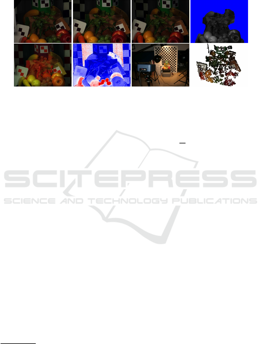
Figure 1: Renderings of the scene used in the experiment. Top row: color RGB renderings from three separate angles and the
mask used for removing calibration markers. Bottom row: false color NIR (Near Infrared), 1000nm bands, acquisition setting
(one of camera locations) and an example 3D point cloud computed from matched keypoints. Note the easy separation of
artificial (plastic) and natural (food) objects on the 1000nm band image, which is much more difficult on visual band range.
Experiment. While there exist a number of dif-
ferent methods that are used for evaluating descrip-
tor performance (see e.g.(Mikolajczyk and Schmid,
2005; Moreels and Perona, 2007)) we argue that in
most practical applications, one is interested either in
extracting 3D scene parameters, or in object recogni-
tion. We focus on the former problem, as it usually
has more general (less application specific) formula-
tion. Also, the quality of 3D estimation verifies de-
scriptors’ sensitivity to actual scene information over
acquisition conditions. The 3D scene estimation from
uncalibrated images is recently becoming a popular
application of image processing methods. It involves
recovering sparse or dense scene 3D point cloud and
camera parameters, from a sequence of images in pro-
cess called Structure From Motion (SFM). For this
task, technique of Bundle Adjustment (see e.g. (Wu
et al., 2011)) is often selected.
We propose a simple evaluation scheme, which
measures the relative error of estimating 3D camera
position. We argue that while individual measures
(e.g. repeatability, stability) are important for quali-
tative assessment of algorithms performance, the fi-
nal application result is very often of key importance.
In case of 3D reconstruction, the quality can be mea-
sured on how well the scene parameters are estimated,
e.g. with reference to ground truth data. Camera posi-
tions are a good benchmark because their precise esti-
mation leads to high quality of the scene point cloud,
and at the same time the position error in 3D is simple
and intuitive. As the scene parameters are estimated
up to a translation and scale factor, the error of cam-
era estimation may be misleading in some cases
3
, we
3
Initial experiments suggested that distortion in relative
position estimation is a better quality predictor of the final
point cloud than absolute position.
propose a performance measure based on error of rel-
ative camera position estimation:
ε =
1
n
p
∑
(i, j),i6= j
k
~
d
ij
−
~
d
′
ij
k
2
(1)
where
~
d
ij
= ~c
j
−~c
i
is the true, and
~
d
′
ij
= ~c
′
j
−~c
′
i
esti-
mated distance between positions of cameras i and j;
n
p
is the number of camera pairs combinations.
We estimate the true positions–ground truth for
the experiments–using semi-automatic point selection
(user assisted with automatic refinement) from cali-
bration markers, inspired and in part similar to ear-
lier work on descriptor comparison (Mikolajczyk and
Schmid, 2005; Moreels and Perona, 2007).
For given range of bands from hyperspectral im-
ages and parametrized descriptor algorithm, we pro-
ceed as follows:
1. Locate interest points and compute descriptors
separately in each image. Only the scene data is
used; calibration markers are masked out (see Fig-
ure 1).
2. For each pair of images, descriptor matches are
computed using Euclidean or Hamming norm (de-
pending on descriptor algorithm) and filtered us-
ing neigborhood ratio r
0
= 0.8.
3. Matched interest points are input to the SFM algo-
rithm, where 3D scene parameters are estimated.
Relative camera positions are measured, and com-
pared with estimated ground truth.
We use VisualSFM (Wu, 2011) software for 3D
scene estimation, as it was easy to integrate with ex-
periment suite and was found to perform well in the
initial tests. The experiments are performed sepa-
rately for different groups of bands (UV, visual, near
infrared range).
VISAPP 2016 - International Conference on Computer Vision Theory and Applications
202

Table 1: Performance of interest point descriptors, as measured with relative camera position estimation. Columns
denote results for given spectral range, rows descriptor algorithms with set parameters (see text). Errors are given
as percentage of a camera model estimated (related to number of cameras identified) and mean of their relative
errors of cameras’ distances measurement (brackets). ‘–’ denotes that camera model estimation did not converge,
in most cases because lack of enough stable feature correspondences.
VIS
a
VIS-B
a
VIS-G
a
VIS-R
a
NIR
b
NIR-1
b
NIR-2
b
NIR-3
b
SIFT-A 100% (1.15) – 100% (0.39) 100% (0.49) – 100% (0.37) – 10% (2.32)
SIFT-B
100% (1.93) 60% (1.91) 100% (0.45) 60% (2.33) 10% (0.47) 100% (1.22) 10% (0.71) 100% (0.66)
SIFT-C
60% (2.00) – 100% (1.04) 100% (3.95) – 100% (0.55) – 10% (2.13)
SURF-100
100% (1.50) 10% (0.47) 100% (0.71) 100% (0.58) 10% (1.00) 100% (2.97) – 100% (0.33)
SURF-300
30% (0.77) – 100% (0.48) 60% (7.80) – 30% (2.33) – 10% (2.35)
SURF-500
30% (2.60) – 60% (1.90) 100% (6.24) – 30% (0.63) – –
BRISK-5
10% (2.54) 10% (2.37) 10% (0.91) 10% (1.16) – 10% (2.22) – –
ORB
10% (2.41) – 10% (2.36) 10% (2.36) – – – –
a
Visual spectral ranges: all 400−700nm, bands 6−63; blue 400−500nm, bands 6− 24; green
500− 590nm, bands 25− 42; red 590− 700nm, bands 64− 82.
b
Near infrared ranges: all 700− 1050nm, bands 64− 127; sub-range 1 is 700− 800nm, bands 64− 82;
sub-range 2 is 800− 900nm, bands 82− 100; sub-range 3 is 900− 150nm, bands 101− 127.
3 RESULTS
Parameters. Interest point descriptor algorithms typ-
ically have a number of parameters, e.g. related
to sensitivity of the detector or type of description
generated. For SIFT method, we use the following
sets of parameters: original values as recommended
in (Lowe, 2004) (SIFT-A); modification of σ =
1.0, contrastThreshold = 0.02,edgeThreshold = 10
based on results of (Sima and Buckley, 2013) (SIFT-
B); and modification of σ = 1.0 as proposed in
(Vakalopoulou and Karantzalos, 2014) as more sensi-
tive version (SIFT-C). For SURF method, we observe
that the main parameter influencing the result is the
Hessian threshold h; implementation (Bradski, 2000)
uses default h = 100 and recommends h ∈ (300, 500),
following that we define three sets of parameters de-
noted as SURF-100, -300, -500. For BRISK method,
we use the threshold parameter t; proposed value of
t = 30 has been observed to generate small number
of keypoints, so we introduce two other values t = 15
and t = 5 to increase sensitivity, final sets are denoted
as BRISK-30, -15 and -5. For ORB method, we use
original recommended parameters (ORB-A), version
with FAST detector instead of Harris (ORB-F), and
version with increased patchSize and edgeThreshold
to p
s
= 51 (ORB-ps), to improve detection on noisy
bands.
As the SFM algorithm is probabilistic in nature,
it was run n = 10 times for each case and the best
model was selected–this correspond to typical usage
scenario.
Test Data. The resulting hyperspectral image set
comprises of five images of dimensions 696 × 520 ×
128, the last dimension corresponds to spectral range
375− 1045nm, with average spectral resolution close
to 5nm and 12 bits of precision. Spectral data at
each pixel is normalized to enhance contrast. For
input to descriptor algorithms, individual bands are
aggregated into groups: (partial) ultraviolet range,
375 − 400nm, bands 1 − 6 and four visual and four
near infrared ranges (see Table 1 notes). The objec-
tive is to reduce noise persistent in individual bands,
while retaining ability to observe performance on dif-
ferent parts of spectral range.
Camera Position Estimation Errors. The results
are presented in Table 1. As it can be expected, esti-
mation of 3D scene parameters from medium-to-low
resolution of hyperspectral camera is a challenging
task for all tested algorithms. In many cases (denoted
‘-’) the number of matched points was not enough
for parameter estimation. In other cases, only some
of cameras were properly identified–to signify this, a
percentage score was added to the error to show how
many relative camera positions could be processed.
Acceptability criteria could be formulated as score of
100% with error close to zero. We note that SIFT
and SURF outperform the BRISK and ORB methods,
with SIFT marginally ahead of SURF in the visual
ranges. Post experiment analysis suggests that per-
formance of ORB suffered because of low number of
detected points, while for BRISK it was high number
of similar matches.
Sensitivity to Spectral Range. Due to varying
degree of blur, noise, and changing scene spectral
characteristics with frequency, the responses of each
feature algorithm have a lot of variance. In particu-
lar the UV range, even with additional light, was too
noisy to produce estimates for any methods. Diffi-
cult range was also whole and middle of near infrared
Performance of Interest Point Descriptors on Hyperspectral Images
203

(NIR and NIR-2), which have a low contrast; how-
ever, when separated the NIR-1 and NIR-3 ranges are
reliable for estimation. This is expected as scene con-
tains both natural and man-made objects, thus their
materials’ reflectances differ in narrow sub-ranges of
the NIR range. Visual range performs best, especially
the VIS-G region, where contrast, sharpness and sig-
nal to noise ratio is at maximum. It is important to
note that the performance in different spectral ranges
is dependent on scene composition, but in general
similar performance can be observed in visual and se-
lected bands of the NIR range.
Sensitivity to Parameters. Standard SIFT-A pa-
rameters perform well, as expected, for visual range.
Increasing sensitivity improves estimation in the far
NIR-3 range, however it must be done with cau-
tion, as can be observed on results of SIFT-B and
-C. Both have been proposed as more sensitive and
hyperspectral-tuned versions, yet the C loses perfor-
mance in the visual range. For SURF, increased sen-
sitivity translates in general to better performance.
Similarly for BRISK, where only the -5 parameter
set was considered, as remaining produced too many
convergence errors. For ORB, modifications of rec-
ommended parameters (ORB-F, ORB-ps) did not pro-
duce improvement in performance.
4 DISCUSSION
Individual Method Performance. While the exact
numbers allow to create ranking list of methods, the
large variability suggests less strict categorization. It
seems that performance of SIFT and SURF is compa-
rable, and better than BRISK and ORB. For the lat-
ter two methods, the performance could be perhaps
improved by exhaustive parameter optimization com-
bined with image preprocessing. This may be im-
portant in practical applications, as ORB and espe-
cially BRISK are much faster than remaining meth-
ods, which can be of use as hyperspectral cameras
produce naturally high volume of data. Increased sen-
sitivity through parameter settings does seem to be a
good strategy; this is similar as reported in (Sima and
Buckley, 2013).
The Characteristics of Hyperspectral Images.
The complex properties of hyperspectral images have
large influence on method performance. While per-
band strategy can be effective in locating various sta-
ble features (e.g. color boundaries in VIS region
or material edges in NIR range), the change of im-
age properties makes the performance of methods un-
even. As for scene composition, there’s a known
effect of scene-dependent performance (cf. conclu-
sions in (Moreels and Perona, 2007)); the adaptation
of methods to characteristics of hyperspectral images
and inclusion of other types of objects will be the sub-
ject of further studies.
Relation to other Works. Our results are in gen-
eral agreement with analysis done for ‘regular’ im-
ages (Mikolajczyk and Schmid, 2005; Moreels and
Perona, 2007). In particular, we affirm the per-
formance and robustness of the SIFT descriptor for
hyperspectral images. This supports the research
done on extending or applying SIFT to hyperspec-
tral images (Xu et al., 2008; Mukherjee et al., 2009;
Ringaby et al., 2010; Dorado-Munoz et al., 2012). We
note, however, that there’s a high chance of attain-
ing similar level of performance with the SURF algo-
rithm. With regards to (Vakalopoulou and Karantza-
los, 2014), we don’t see their level of error when
using standard SIFT or SURF parameters in the vi-
sual spectral range. On the contrary, this is the re-
gion where both methods perform quite well; this is
in fact expected, as bands in visual range are close to
grayscale images used to derive original parameters.
One possible reason for this difference could be some
unique properties of the capturing equipment or imag-
ined scenes used by (Vakalopoulou and Karantzalos,
2014). Our study is less investigative in the inter-
play of different parameters than (Sima and Buckley,
2013), as we have not one, but four different parame-
ter sets to analyze.
Conclusions. We’ve presented a performance
analysis of several interest point descriptor methods
as applied to hyperspectral images in a novel set-
ting. We show the SIFT and SURF both produce quite
good results across bands. Application of BRISK and
ORB, while faster, did not result in stable 3D estima-
tion from this type of images. For improving perfor-
mance of descriptors on hyperspectral data, we rec-
ommend increasing sensitivity through parameter set-
tings, and location of informative spectral ranges, e.g.
with prior knowledge or additional preprocessing.
ACKNOWLEDGEMENTS
This work has been supported by the project ‘Rep-
resentation of dynamic 3D scenes using the Atomic
Shapes Network model’ financed by National Science
Centre, decision DEC-2011/03/D/ST6/03753.
REFERENCES
Bay, H., Ess, A., Tuytelaars, T., and Gool, L. V. (2008).
Speeded-up robust features (SURF). Computer Vision
VISAPP 2016 - International Conference on Computer Vision Theory and Applications
204

and Image Understanding, 110(3):346 – 359. Simi-
larity Matching in Computer Vision and Multimedia.
Bradski, G. (2000). The OpenCV library. Dr. Dobb’s Jour-
nal of Software Tools.
Brown, M. and Susstrunk, S. (2011). Multi-spectral SIFT
for scene category recognition. In 2011 IEEE Con-
ference on Computer Vision and Pattern Recognition
(CVPR), pages 177–184.
Dorado-Munoz, L., Velez-Reyes, M., Mukherjee, A., and
Roysam, B. (2012). A vector SIFT detector for in-
terest point detection in hyperspectral imagery. IEEE
Transactions on Geoscience and Remote Sensing,
50(11):4521–4533.
Leutenegger, S., Chli, M., and Siegwart, R. Y. (2011).
BRISK: Binary robust invariant scalable keypoints. In
Proceedings of the International Conference on Com-
puter Vision (ICCV).
Lowe, D. (2004). Distinctive image features from scale-
invariant keypoints. International Journal of Com-
puter Vision, 60(2):91–110.
Mikolajczyk, K. and Schmid, C. (2005). A perfor-
mance evaluation of local descriptors. IEEE Trans-
actions on Pattern Analysis and Machine Intelligence,
27(10):1615–1630.
Moreels, P. and Perona, P. (2007). Evaluation of features
detectors and descriptors based on 3d objects. Inter-
national Journal of Computer Vision, 73(3):263–284.
Mukherjee, A., Velez-Reyes, M., and Roysam, B. (2009).
Interest points for hyperspectral image data. IEEE
Transactions on Geoscience and Remote Sensing,
47(3):748–760.
Ringaby, E., Ahlberg, J., Wadstr¨omer, N., and Forss´en, P.-E.
(2010). Co-aligning aerial hyperspectral push-broom
strips for change detection. In Proc. SPIE, volume
7835, pages 78350Y–78350Y–7.
Rublee, E., Rabaud, V., Konolige, K., and Bradski, G.
(2011). ORB: an efficient alternative to SIFT or
SURF. In Proceedings of the International Confer-
ence on Computer Vision (ICCV).
Sima, A. A. and Buckley, S. J. (2013). Optimizing SIFT
for matching of short wave infrared and visible wave-
length images. Remote Sensing, 5(5):2037–2056.
Vakalopoulou, M. and Karantzalos, K. (2014). Automatic
descriptor-based co-registration of frame hyperspec-
tral data. Remote Sensing, 6(4):3409–3426.
Wu, C. (2011). VisualSFM: A visual structure from motion
system. http://ccwu.me/vsfm/.
Wu, C., Agarwal, S., Curless, B., and Seitz, S. (2011). Mul-
ticore bundle adjustment. In Computer Vision and Pat-
tern Recognition (CVPR), 2011 IEEE Conference on,
pages 3057–3064.
Xu, Y., Hu, K., Tian, Y., and Peng, F. (2008). Classifica-
tion of hyperspectral imagery using SIFT for spectral
matching. In 2008 Congress on Image and Signal Pro-
cessing, CISP ’08., volume 2, pages 704–708.
Performance of Interest Point Descriptors on Hyperspectral Images
205
