Eco-routing: An Ant Colony based Approach

Ahmed Elbery

, Hesham Rakha

, Mustafa Y. ElNainay

Wassim Drira

and Fethi Filali

Dept. of Computer Science, Virginia Tech, Blacksburg, VA, U.S.A.

Civil and Environmental Engineering, Virginia Tech, 3500 Transportation Research Plaza, 24061, Blacksburg, VA, U.S.A.

Dept. of Computer and Systems Eng, Alexandria University, Alexandria, Egypt

Qatar Mobility Innovations Center, PO Box 210531, Qatar Science and Technology Park, Doha, Qatar

Keywords: Eco-routing, Ant Colony, Fuel Consumption, Emissions, Travel Time, Vehicle Routing, ITS.

Abstract: Global warming, environmental pollution, and fuel shortage are currently major worldwide challenges. Eco-

routing is one of several tools that attempt to address this challenge by minimizing network-wide vehicle fuel

consumption and emission levels. Eco-routing systems select the most environmentally friendly route. The

subpopulation feedback eco-routing (SPF-ECO) algorithm that is implemented in the INTEGRATION

software can produce a reduction in fuel consumption levels by approximately 17%. However, in some cases,

due to delayed updates or the lack for updates, its performance degrades. In this paper, we propose the ant

colony based eco-routing technique (ACO-ECO), which is a novel feedback eco-routing and cost updating

algorithm to overcome these shortcomings. In the ACO-ECO algorithm, real-time performance measures on

various roadway links are shared. Vehicles build their minimum path routes using the latest real-time

information to minimize their fuel consumption and emission levels. ACO-ECO is also able to capture

randomness in route selection, pheromone updating, and pheromone evaporation. The results show that the

ACO-ECO algorithm and SPF-ECO have similar performances in normal cases. However, in the case of link

blocking, the ACO-ECO algorithm reduces the network-wide fuel consumption and CO

emission levels in

the range of 2.3% to 6.0%. It also reduces the average trip time by approximately 3.6% to 14.0%.

1 INTRODUCTION

The environmental and economic impact of the

transportation sector has necessitated research in

recent years because the transportation sector is an

important source of the major current challenges,

including: global warming, energy and fuel shortage,

and environmental pollution. In 2008, the U.S.

Department of Energy mentioned in (U.S. Dept.

Energy 2008) that approximately 30% of the fuel

consumption in the U.S. is consumed by vehicles

moving on the roadways. In addition, about one-third

of the U.S. carbon dioxide (



) emissions comes

from vehicles (U.S. E.P Agency 2006). The 2011

McKinsey Global Institute report estimated savings

of “about $600 billion annually by 2020” in terms of

fuel and time saved by helping vehicles avoid

congestion and reduce idling at red lights or left turns.

From the drivers’ perspective, drivers usually

select routes that minimize their costs such as travel

time or travel distance. However, the minimum time

or distance routes do not necessarily minimize the

fuel consumption or emission levels (Barth,

Boriboonsomsin et al. 2007, Ahn and Rakha 2008).

There are many cases where the minimum time routes

result in higher fuel consumption levels such as high-

speed routes; despite the time reduction that could be

achieved, the higher speed routes may produce higher

fuel consumption levels due to the higher vehicle

speeds, route grades or longer distance. Also, shorter

distance routes can result in higher fuel consumption

if the speed is too low or if the route has many

intersections that result in numerous deceleration and

acceleration manoeuvres. Selecting the minimum time

or minimum distance routes is simple compared to

finding the minimum fuel consumption routes. The

fuel consumption depends on many parameters such as

distance, travel time, route grades, congestion level,

vehicle characteristics, and the driving behaviour.

Researchers have proposed several models for the

estimation of vehicle fuel consumption and emission

levels. These models can be classified into two

classes; macroscopic models (Brzezinski 1999, ARB

2007) and microscopic models (Barth 2000, Rakha,

Ahn et al. 2004). In macroscopic models, the average

link speeds are used to estimate the fuel consumption

and emission levels for each link. This class is

Elbery, A., Rakha, H., ElNainay, M., Drira, W. and Filali, F.

Eco-routing: An Ant Colony based Approach.

In Proceedings of the International Conference on Vehicle Technology and Intelligent Transport Systems (VEHITS 2016), pages 31-38

ISBN: 978-989-758-185-4

characterized by its simplicity but has a limited

accuracy because it ignores the speed and the

acceleration impacts on fuel consumption levels.

Meanwhile, microscopic models overcome this

limitation using instantaneous speed and acceleration

levels to estimate the fuel consumption and emission

levels. Consequently, microscopic models provide

higher accuracy at the cost of model complexity.

Eco-routing (Ericsson, Larsson et al. 2006) was

developed to select the route that minimizes vehicle

fuel consumption levels between an origin and

destination. In a feedback system, Eco-routing

depends on the vehicle and route characteristics as

well as its ability to report this information to a traffic

management center (TMC) that updates the routing

information, rebuilds the routes, and sends the new

routes to vehicles traversing the network.

Eco-routing is a promising navigation technique

because it results in a significant reduction in fuel

consumption and emission levels. However, through

some improvements, the Eco-routing system can be

further enhanced to produce additional fuel

consumption and emission savings.

In this paper, we first study the Eco-routing

performance and show that in some cases its

performance may not be optimum. Subsequently,

based on this, we propose an ant colony Eco-routing

(ACO-ECO) algorithm that employs the ant colony

optimization algorithms (Dorigo and Birattari 2010).

Due to the major differences between the ant colony

and the transportation network, the ant colony

algorithms are not directly applied to select the best

routes, however, they are used to optimize the route

selection process by optimizing the route selection

updating. Finally, we compare the proposed approach

to the subpopulation feedback Eco-routing algorithm

(SPF-ECO) (Rakha, Ahn et al. 2012).

The remainder of this paper is organized as

follows. An overview of the Eco-routing literature

and the subpopulation feedback assignment Eco-

routing (SPF-ECO) algorithm is introduced. This is

followed by outlining the main problems with the

SPF-ECO algorithm. Subsequently, an overview of

the ant colony optimization is presented. After that,

the proposed approach (ACO-ECO) is described.

Subsequently, the simulation results that compare the

ACO-ECO to the SPF-ECO are presented and

discussed. Finally, the study conclusions are presented

together with recommendations for further research.

2 ECO-ROUTING LITERATURE

In 2006, Ericsson et al. proposed the Eco-routing in

(Ericsson, Larsson et al. 2006) where they presented

a comprehensive study that provides optimal route

choices for lowest fuel consumption. The fuel

consumption measurements are made through the

extensive deployment of sensing devices in the street

network in the city of Lund, in Sweden. This study

showed that about 46% of the trips were not made on

the most fuel-efficient route. And approximately 8%

of the fuel consumption could be saved on average

using the most fuel-efficient routes. In 2007, Barth et

al. (Barth, Boriboonsomsin et al. 2007) combined

sophisticated mobile-source energy and emission

models with route minimization algorithms to

develop navigation techniques that minimize energy

consumption and pollutant emissions. They

developed a set of cost functions that include the fuel

consumption and the emission levels for the road

links. In 2007, Ahn and Rakha (Ahn and Rakha 2007)

showed the importance of route selection on the fuel

consumption and environmental pollution reduction,

by demonstrating through field tests that an emission

and energy optimized traffic assignment could reduce





emissions by 14 to 18%, and fuel consumption

by 17 to 25% over the standard user equilibrium and

system optimum assignment. Later in 2012, Rakha et

al. (Rakha, Ahn et al. 2012), introduced a stochastic,

multi-class, dynamic traffic assignment framework

for simulating Eco-routing using the

INTEGRATION software (Rakha Last Access Feb.

2016). They demonstrated that fuel savings of

approximately 15% using two scenarios were

achievable. In (Boriboonsomsin, Barth et al. 2012),

the authors developed an Eco-routing navigation

system that selects the fuel-efficient routes based on

both historical and real-time traffic information.

2.1 Subpopulation Feedback

Eco-routing

In this section, we will describe in details the

subpopulation feedback assignment Eco-Routing

SPF-ECO (Rakha, Ahn et al. 2012) implemented in

the INTEGRATION software. INTEGRATION uses

the VT-Micro model (Rakha, Ahn et al. 2004) for

calculating the fuel consumption rate 

(



)

in / for

each vehicle as shown in Equation (1).



(



)













,



















≥0





,



















<0



(1)

VEHITS 2016 - International Conference on Vehicle Technology and Intelligent Transport Systems

Here 

,

are model regression coefficients at

speed exponent  and acceleration exponent, 

,

are model regression coefficients at speed exponent 

and acceleration exponent,  is the instantaneous

vehicle speed in (km/h), and  is the instantaneous

vehicle acceleration (km/h/s).

An important characteristic of INTEGRATION is

its time granularity which is a deci-second resolution.

This granularity enables it to accurately calculate the

fuel consumption and emissions based on

instantaneous speed and acceleration levels.

In SPF-ECO, when the vehicle enters a new link.

The vehicle’s fuel consumption and emission levels

are reset to zero for the new link. Subsequently, the

SPF-ECO algorithm periodically calculates the fuel

consumption and emissions for each vehicle using

Equation (1). For each vehicle, the estimated fuel

consumption and emission levels are accumulated

until the vehicle traverses the link. When a vehicle

leaves a link, it submits its fuel consumption cost for

this link to the traffic management center (TMC),

which updates the link fuel consumption using some

smoothing techniques. Subsequently,

INTEGRATION periodically rebuilds the routes for

each origin-destination pair at a frequency specified

by the user. Subsequently, vehicles use the latest

paths when looking identifying the next link along the

route. This mechanism has three main shortcomings

that are discussed in this section.

2.1.1 Fixed Cost for Empty Links

Assume that a link 



was loaded with a high traffic

flow that resulted in congestion on this link. This

congestion will result in a lower speed and increasing

the acceleration/deceleration noise. Consequently,

increasing the fuel consumption and emission levels

on this link. At a certain time, the SPF-ECO system

will re-route vehicles to another route that reduces the

route cost. Since the vehicles on 



have been exposed

to the congestion, the link fuel consumption will be

very high after these vehicles leave the link. As the

system re-routes vehicles to other routes, the link will

not be loaded by vehicles until the routing

information changes. Consequently, the cost of





will continue to be high while it is actually

decreasing. This lag in the system is typical of any

feedback control system and will result in vehicles

using sub-optimal routes. Consequently, increasing

the network-wide fuel consumption levels.

2.1.2 Fixed Cost for Blocked Links

A reverse situation can take place in case of blocking

a link (for example due to an incident). In this case

the vehicles that were not blocked will have a low fuel

consumption level, and will report it when leaving the

link. The SPF-ECO will maintain a low cost for this

link as long as the link is blocked since there is no

vehicle leaving the link to update the information on

this link. Consequently, the SPF-ECO will continue

to use this route and load more vehicles to this link

resulting in higher fuel consumption and emission

levels.

2.1.3 Delayed Updates

The third point is that the updates are only sent when

a vehicle leaves a link. For long links and/or low-

speed links, the link travel time is relatively long.

Consequently, the information used to update the

SPF-ECO routing might be obsolete and may not

reflect the current state of the link. This inaccurate

routing information might result in incorrect routing

decisions and hence increase the fuel consumption

level.

In the proposed approach, we solve these

problems by utilizing ant colony techniques to update

the link cost function (the fuel consumption level in

this application).

3 ANT COLONY OPTIMIZATION

Ant colony optimization (Dorigo and Birattari 2010)

is a branch of the larger field of swarm intelligence

(Blum and Li 2008). Swarm intelligence studies the

behavioural patterns of social insects such as bees,

termites, and ants in order to simulate these processes.

Ant colony optimization is a meta-heuristic iterative

technique inspired from the foraging behaviour of

some ant species. In the ant colony, ants walking to

and from a food source deposit a substance called

pheromone on the ground. In this way, ants mark the

path to be followed by other members of the colony.

The shorter the path, the higher the pheromone on that

route, and consequently, the preferable this route is.

The other ant colony members perceive the presence

of pheromone and tend to follow paths where

pheromone concentration is higher. Ant colony

optimization exploits a similar mechanism for solving

some optimization problems.

In this paper, we use the same ant colony concept

to optimize the fuel consumption and emission cost

for a transportation network. Vehicles are employed

as artificial ants, the pheromone is considered to be

the inverse of the fuel consumption cost for each link.

Each artificial ant periodically deposits the

Eco-routing: An Ant Colony based Approach

pheromone by updating the fuel consumption cost for

the link it is traversing.

There are many variants of ant colony

optimization. However, all of them share the same

idea described earlier. The main steps in each

iteration are: 1) construct the solutions, 2) conduct an

optional local search step, and 3) update pheromones.

The ant colony system does not specify how these

three steps are scheduled and synchronized, the

system leaves these decisions to the algorithm

designer (Blum 2005). In the solution construction

step, artificial ants construct a feasible solution and

add it to the solution space. The system starts with an

empty solution space, the ants start at the nest, and

each ant probabilistically chooses a solution





between a set of paths







,



,…





to reach the

food source. To choose between these paths, each ant

uses the probability 



computed in Equation (2).





=



∑











(2)

Where 



is the amount of pheromone on path



This probabilistic behavior for route selection

guarantees the exploration of more feasible solutions

and avoids converging to local ones.

The pheromone updating takes place while the

ants are moving, where they deposit the pheromone

on their paths. Also, as time passes, the pheromone

evaporates based on an evaporation factor.

Subsequently, after each iteration, the phenome is

updated according to Equation (3).





(

1−

)





+









(3)

Where  is the number of ants that traverse a

link, and 



is the amount of pheromone deposited

by ant. After the solution construction and before

the pheromone updating, the local search step can be

carried out to improve the solution. This step is

optional and problem specific.

In the proposed approach, we utilize these steps to

achieve our objective of minimizing the fuel

consumption and consequently the pollutant

emissions.

4 ANT COLONY BASED

ECO-ROUTING (ACO-ECO)

This section presents the proposed approach (ACO-

ECO) and describes its operation in details. In ACO-

ECO, the ant colony techniques will be applied to

optimize the fuel consumption and emissions in the

transportation network. The vehicles are the artificial

ants, and the pheromone is the inverse of the fuel

consumption. Because of the major differences

between the ant colony system and the transportation

network, we introduce some variations to ant colony

techniques to tailor it to the specific application. The

ACO-ECO uses a number of steps that are described

here.

4.1 Initialization

This phase initializes the cost associated with the

various links. Because initially the links are free, the

cost of each link is initialized to the free flow speed

fuel consumption using equation (1).

4.2 Route Construction

This phase starts directly after the initialization phase

and is repeated periodically and was defined to be 60

seconds in this application. In this phase, the ACO-

ECO builds the minimum path based on the cost of

each link. When the vehicle leaves a route link, it

searches the tree to find its next link.

The probabilistic route selection (introduced by

Equation (2)) is an important mechanism in ant

colony algorithms to search all the available routes.

However, this mechanism as described in Equation

(2) cannot be applied in vehicular route selection

because it is not realistic. As mentioned earlier,

drivers try to select routes that minimize their cost,

while this probabilistic selection assigns a random

route to each vehicle based on the route’s pheromone

level (route cost) relative to that for all other routes.

Using this equation, and due to the randomness, a

vehicle might be assigned a very high-cost route

which is not realistic, and is not consistent with the

driver behaviour when selecting routes.

Consequently, it will result in a higher fuel

consumption level. So, we use another technique to

introduce some limited randomness into the route

selection mechanism while maintaining the error

within a given predefined margin. An error factor is

configured for the network. This error factor (α) is

used to add some error to the cost of the links,

subsequently to the tree building and the route

selection algorithms. The error value added to the link

cost is a randomly selected point from the standard

normal distribution(0,σ), where σ is the standard

deviation andσ=α._. In this way, we

have a grantee that 95.45% of the link costs are

within

(

1±2α

)

._. Which means that by

controlling the error factor  we can control the

VEHITS 2016 - International Conference on Vehicle Technology and Intelligent Transport Systems

randomness level within the route selection

algorithm.

4.3 Pheromone Update

In this phase, two updating processes take place.

Pheromone deposition where ants deposit pheromone

to indirectly communicate the route preference to the

following ants. And the pheromone evaporation,

where the pheromone level on each link decays with

time.

4.3.1 Pheromone Deposition

In the vehicular network, each vehicle sends the cost

it experienced on a link to the TMC, and

consequently, the link cost is updated in the routing

algorithm. In the SPF-ECO, the vehicles only submit

the link cost when leaving the link. The advantage of

this method is the small number of updates being sent

on the network and consequently the low network

overhead. But on the other hand, it results in delayed

updates and fixed cost for empty or blocked links as

mentioned earlier.

In contrast to the SPF-ECO, the ACO-ECO

overcomes these issues by enabling vehicles to

submit multiple updates while traveling the link.

These updates can be sent periodically either time-

based or distance-based. Using time-based updating,

the vehicles have a predefined maximum updating

interval. The vehicles should send their estimation

for the link cost each  seconds. This cost updating

method can control the number of updates that are

sent over the network. However, it has an important

drawback; for low speed links or blocked links, the

vehicles will send many unnecessary updates.

Another drawback is for short length links and/or

high speed links, this time interval may be longer

than the link traversal time. Consequently, no updates

would be sent for these links. This drawback can be

overcome by setting  to a value that is shorter than

the minimum link travel time in the network,

however, this will result in many unnecessary updates

for long links or low speed links.

Another way to submit the link cost updates is the

distance based updating, where the vehicles should

submit an update every distance  it traverses on the

link. In contrast to the time based updating, the

distance based method limits the number of updates

for each link. But on the other hand, for blocked links,

the updates will not be sent and consequently, the cost

will be fixed for blocked links resulting in the same

problem as the SPF-ECO algorithm.

Consequently, a compromise approach is

proposed, which combines both the time- and

distance-based updating to take advantage of the

merits of each approach. Also, we used the end of the

link updating where the vehicle sends an update when

it leaves the link. To estimate the link fuel

consumption, the ACO-ECO algorithm defines the

maximum time interval  and the maximum

distance to report conditions. When any of these

conditions is met, the vehicle submits a new update

quantifying its estimation for the overall link cost, and

then resetting its time and distance counter. To

calculate the fuel it consumed, the ACO-ECO

periodically estimates the fuel consumption rate using

the VT-Micro model in Equation (1). And then uses

Equation (4) to accumulate the total fuel consumed in

the previous interval.

=

(



)

.∆





(4)

Where 

(



)

is the VT-Micro model instantaneous

fuel consumption rate, and ∆is the fuel consumption

calculation interval which is typically 0.1 seconds in

INTEGRATION. Whenever either  or  is reached,

the ACO-ECO estimates the overall link fuel

consumption 



as shown in Equation (5).





.





(5)

Where is the distance traveled in the previous

period in meters(≤), and the link length in

meters. This calculation assumes that the conditions

on the remainder of the link will continue as was

observed by the vehicle.

4.3.2 Pheromone Evaporation

To overcome the fixed cost problem for empty links,

the cost of these links must be updated when the TMC

has not received updates for a period of time. In an

ant colony, if no pheromone is deposited for a long

time, the link pheromone level will decay towards

zero due to the evaporation, this is an indication of the

low preference for that route. In a transportation

network, not receiving an update about a link for a

long time, indicates that this link is empty.

Consequently, the cost of this link must be updated

toward the free flow speed cost(





). So, in this

case, the TMC updates the cost as follows. First, it

finds the minimum updating interval (



) for the link.

This value is the minimum of three parameters; the

updating interval (T), the link travel time at free-flow

speed, and the updating interval in case of distance

based updating. These parameters are shown in

Equation (6). The rationale is that after receiving an

Eco-routing: An Ant Colony based Approach

update, the next vehicle will send an update in case of

one of three situations; it reaches its updating

interval, it reaches its updating distance, or it ends

the link.





=,























(6)

Where  is the updating interval,  is the updating

distance, 



is the link length and 





is the free-flow

speed of the link.

Subsequently, the ACO-ECO algorithm estimates

the overall link cost 



as shown in Equation (7). This

evaporation technique results in exponential

increasing or decreasing in the link cost towards the

free-flow speed cost.





=



−

∆









−









(7)

Where 





is the free-flow speed fuel

consumption estimate for the link, and ∆ is the

evaporation interval after which the evaporation

process should be performed for the link cost if no

updates were received.

5 SIMULATION RESULTS

In this section, we compare the proposed approach

ACO-ECO to the SPF-ECO for different traffic rates

using the INTEGRATION software (Rakha Last

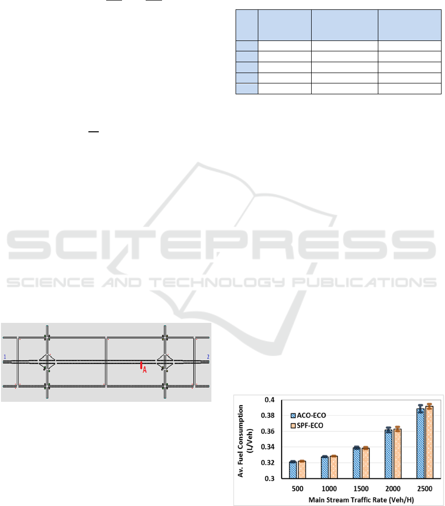
Access Feb. 2016). The network shown in Figure 1

is used for comparing the two approaches.

Figure 1: Road Network used in Simulation.

The network consists of 10 zones with the main

highway (center horizontal road) between zone 1 and

zone 2, and two arterial roads (side roads). The

network size is 3.5 km x 1.5 km. The free-flow speeds

are 110 and 60 km/h for the highway and arterial

roads, respectively. The highway has 3 lanes in each

direction while the other roads have only 2 lanes in

each direction. Regarding the origin-destination

traffic demands (O-D demands), we use 5 different

scenarios, as shown in Table 1. The main traffic

stream is the traffic between zone 1 and 2 for each

direction, the side traffic streams are between each

two other zone pairs. This traffic rate is generated for

half an hour, and the simulation runs for 4500 seconds

to ensure that all the vehicles complete their trips.

Table 1: Origin-Destination Traffic Demand Configuration.

Main

Demand

(Veh/h)

Secondary

Demand

(Veh/h)

Total no.

vehicles

(Veh)

1 500 50 1600

2 1000 75 2650

3 1500 100 3700

4 2000 125 4750

5 2500 150 5800

The comparison is done in two cases; the normal

operation (no incident) case where there is no link

blocking, and in the case of blocking due to an

incident (link blocking case). For each case, we run

each traffic assignment technique (ACO-ECO, and

SPF-ECO) 20 times with different seeds to consider

the output variability due to randomization. This is

repeated for each of the five O-D demand

configurations. The error factor is set for both

techniques to 1%. For the ACO-ECO parameters, the

maximum update interval  is 180 seconds, and the

maximum update distance  is 750 meter.

5.1 Normal Operation Scenarios

For the normal operation scenarios, the results show

no significant differences between the ACO-ECO and

the SPF-ECO for average fuel consumption levels, as

shown in Figure 2. The figure also shows that as the

traffic demand increases, the average fuel

consumption and the average trip time increases due

to the higher congestion levels. Moreover, the results

show the same behaviour for the average trip time,

theCO



and 



emissions levels, where ACO-ECO

has no significant effect on any of them.

Figure 2: Average Fuel Consumption (L/Veh).

Regarding the  emission, the ACO-ECO has a

higher emission level as shown in Figure 3.

VEHITS 2016 - International Conference on Vehicle Technology and Intelligent Transport Systems

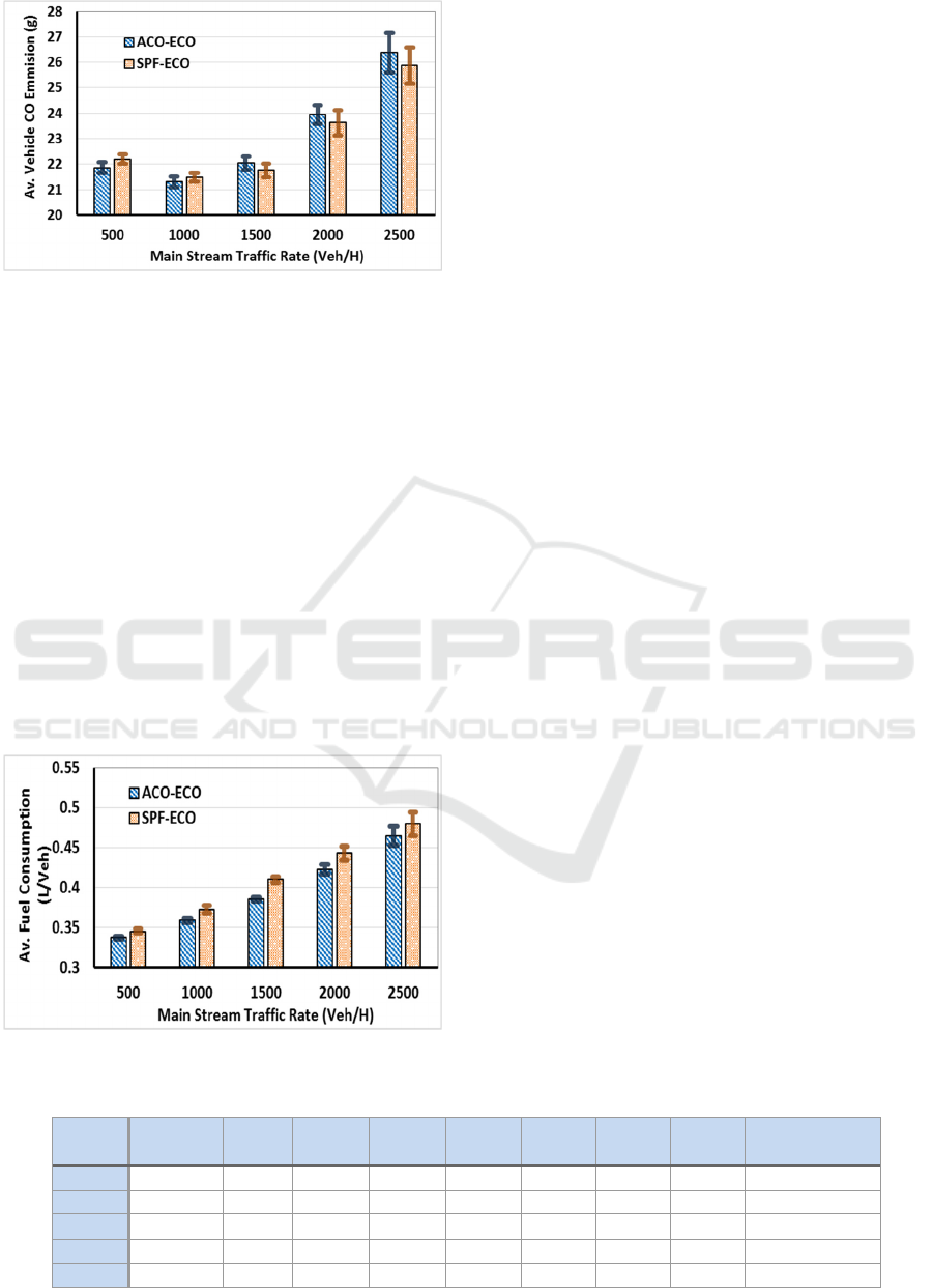
Figure 3: Average Vehicle CO Emission.

5.2 Incident Scenarios

To simulate the link blocking in the network, we

configured an incident on the highway from zone 1

and 2 at point (A) marked in Figure 1, the incident

does not affect the other direction from zone 2 to zone

1. This incident occurs 10 minutes after starting the

simulation and blocks 50% of the highway (1.5 lanes)

for 5 minutes. Then the blocking is reduced to 25% of

the highway for the next 10 minutes, then the incident

is completely removed and the highway works with

its full capacity.

Figure 4 shows the fuel consumption in case of an

incident. The figure demonstrates that the ACO-ECO

algorithm reduces the average fuel consumption level

for all traffic demands. The reduction ranges between

2.3% to 6% compared to the SPF-ECO.

Figure 4: The Average Fuel for the Link Blocking Scenario.

These results show the ability of ACO-ECO to

reduce the fuel consumption level and the trip time in

addition to all the time-related measurements. ACO-

ECO also succeeds in reducing the pollutant

emissions in most cases.

Table 2 shows the percentage reduction attributed

to the ACO-ECO for both fuel consumption, different

emissions, and different time-related measurements.

For instance, the fuel consumption is reduced by 6%

in the moderate traffic scenario and this reduction

ratio decreases as the traffic demand increases. This

also applies for the CO



emissions and the time-

related measurements. The reason is that as the traffic

demand increases, the congestion increases and thus

affects all the alternative routes, which limits the

ACO-ECO ability to recover from the congestion.

To find the significance of the reduction made by

ACO-ECO, analysis of variance (ANOVA) is

employed to compare means of ACO-ECO to that of

SPF-ECO.

The hypotheses are:-

• Null hypothesis: the means for both algorithms

are equal (



:



=



)

• The alternate hypothesis: the means are not

equal(



∶







We applied this ANOVA for the fuel consumption

results in the lowest traffic rate. Given this scenario

has the lowest reduction in fuel consumption. The

result shows that p-value is less than 0.0001. Which

gives a strong evidence to reject the null hypothesis.

And shows the significance of the reduction mad by

the ACO-ECO. And, since the lowest reduction level

is significant, we can conclude that the higher levels

for other configuration are also significant.

Table 2 also, shows some rare cases where the

some emissions increase in due to the use of ACO-

ECO. For instance, CO and NOx emissions increased

in case high traffic rates.

6 CONCLUSIONS

We propose an ACO-ECO traffic assignment

technique that is inspired from the ant colony

Table 2: Percent of Reduction Made by ACO-ECO over SPF-ECO in case of Link Blocking.

Traffic

rate

Fuel CO

CO HC NO

Trip

time

Stop

delay

Accel.

noise

Accel./Decel.

delay

500 2.37 2.29 3.75 3.71 1.60 3.64 4.04 1.87 12.02

1000 3.72 3.86 1.05 1.73 0.91 8.83 19.04 4.90 21.97

1500 6.06 6.42 -1.51 0.38 0.24 14.98 27.68 5.28 25.43

2000 4.57 4.75 0.49 2.19 0.11 12.66 19.75 4.91 16.84

2500 3.09 3.32 -2.10 -0.58 -0.75 7.11 15.39 1.61 11.34

Eco-routing: An Ant Colony based Approach

optimization algorithm. ACO-ECO attempts to

enhance the SPF-ECO algorithm that is currently

implemented in the INTEGRATION software. These

enhancements include cases in which the links are

blocked or no vehicles traverse the link. ACO-ECO

employs the ant colony techniques to minimize the

fuel consumption and emission levels. It uses the

route construction to build routes and assign them to

vehicles, it also applies pheromone deposition and

pheromone evaporation to update the route link costs.

These ant colony techniques are customized to be

suitable for transportation networks. In the case of

normal operation, the ACO-ECO performance is

similar to the SPF-ECO. While for link blocking

scenarios, the ACO-ECO reduces the fuel

consumption, average trip time, stopped delay, and

most of the emission levels. An important advantage

of the ACO-ECO is its flexibility; where its

parameters (error factor, maximum updating time,

maximum updating distance, and evaporation

interval) can be tuned in order to achieve better

performance. The fine tuning and testing of these

parameters are an important future extension of the

work presented in this paper.

Another future research is to study the effect of

each of the new updating methods on the network

traffic and studying the trade-off between the

reduction in the fuel consumption and emission levels

and the communication network traffic load. The

market penetration rate is an effective and important

parameter that should be studied. Also, it is important

to study the effect of the communication network on

the ACO-ECO performance.

ACKNOWLEDGEMENTS

This effort was jointly funded by the TranLIVE and

MATS University Transportation Centers and by

NPRP Grant 5-1272-1-214 from the Qatar National

Research Fund (a member of the Qatar Foundation).

REFERENCES

Ahn, K. and H. Rakha (2007). Field evaluation of energy

and environmental impacts of driver route choice

decisions. Intelligent Transportation Systems

Conference, 2007. ITSC 2007. IEEE, IEEE.

Ahn, K. and H. Rakha (2008). "The effects of route choice

decisions on vehicle energy consumption and

emissions." Transportation Research Part D: Transport

and Environment 13(3): 151-167.

ARB, C. A. R. B. (2007). " User’s Guide to EMFAC,

Calculating emission inventories for vehicles in

California.".

Barth, M., An, F., Younglove, T., Scora, G., Levine, C.,

Ross, M., and Wenzel, T. (2000). "Comprehensive

modal emission model (CMEM) version 2.0 user’s

guide. Riverside, Calif.".

Barth, M., et al. (2007). Environmentally-Friendly

Navigation. Intelligent Transportation Systems

Conference, 2007. ITSC 2007. IEEE.

Blum, C. (2005). "Ant colony optimization: Introduction

and recent trends." Physics of Life reviews 2(4): 353-

373.

Blum, C. and X. Li (2008). Swarm intelligence in

optimization, Springer.

Boriboonsomsin, K., et al. (2012). "Eco-Routing

Navigation System Based on Multisource Historical

and Real-Time Traffic Information." Intelligent

Transportation Systems, IEEE Transactions on 13(4):

1694-1704.

Brzezinski, D. J., Enns, P, and Hart, C. (1999). "Facility-

specific speed correction factors. MOBILE6

Stakeholder Review Document." U.S. Environmental

Protection Agency (EPA).

Dorigo, M. and M. Birattari (2010). Ant Colony

Optimization. Encyclopedia of Machine Learning. C.

Sammut and G. Webb, Springer US: 36-39.

Ericsson, E., et al. (2006). "Optimizing route choice for

lowest fuel consumption – Potential effects of a new

driver support tool." Transportation Research Part C:

Emerging Technologies 14(6): 369-383.

Rakha, H. ( Last Access Feb. 2016). INTEGRATION Rel.

2.40 for Windows - User's Guide, Volume I:

Fundamental Model Features. https://sites.google.com

/a/vt.edu/hrakha/.

Rakha, H., et al. (2004). Emission model development using

in-vehicle on-road emission measurements. Annual

Meeting of the Transportation Research Board,

Washington, DC.

Rakha, H., et al. (2012). "INTEGRATION Framework for

Modeling Eco-routing Strategies: Logic and

Preliminary Results." International Journal of

Transportation Science and Technology 1(3): 259-274.

U.S. Environ Protection Agency (2006). Inventory of U.S.

greenhouse gas emissions and sinks. 1990–2006,

Washington, DC, .

U.S. Dept. Energy (2008). Annual Energy Outlook 2008,

With Projection to 2030,. Energy Inf. Admin.,

Washington, DC, Rep. DOE/EIA-0383(2008),.

VEHITS 2016 - International Conference on Vehicle Technology and Intelligent Transport Systems