
Efficient Evidence Accumulation Clustering for Large Datasets
Diogo Silva
1
, Helena Aidos
2
and Ana Fred
2
1
Portuguese Air Force Academy, Sintra, Portugal
2
Instituto de Telecomunicac
˜
oes, Instituto Superior T
´
ecnico, Lisboa, Portugal
Keywords:
Clustering Methods, EAC, K-Means, MST, GPGPU, CUDA, Sparse Matrices, Single-Link.
Abstract:
The unprecedented collection and storage of data in electronic format has given rise to an interest in automated
analysis for generation of knowledge and new insights. Cluster analysis is a good candidate since it makes as
few assumptions about the data as possible. A vast body of work on clustering methods exist, yet, typically,
no single method is able to respond to the specificities of all kinds of data. Evidence Accumulation Clustering
(EAC) is a robust state of the art ensemble algorithm that has shown good results. However, this robustness
comes with higher computational cost. Currently, its application is slow or restricted to small datasets. The
objective of the present work is to scale EAC, allowing its applicability to big datasets, with technology
available at a typical workstation. Three approaches for different parts of EAC are presented: a parallel GPU
K-Means implementation, a novel strategy to build a sparse CSR matrix specialized to EAC and Single-Link
based on Minimum Spanning Trees using an external memory sorting algorithm. Combining these approaches,
the application of EAC to much larger datasets than before was accomplished.
1 INTRODUCTION
The amount and variety of data that exists today has
sparked the interest in automated analysis for gener-
ation of knowledge. Thus, clustering algorithms are
useful to explore the structure of data by organizing it
into clusters. Many clustering algorithms exist (Jain,
2010), but usually they are data dependent. Inspired
by the work on sensor fusion and classifier combi-
nation, ensemble approaches (Fred, 2001; Strehl and
Ghosh, 2002) have been proposed to address the chal-
lenge of clustering a wider spectrum of datasets.
The present work builds on the Evidence Accu-
mulation Clustering (EAC) framework presented by
(Fred and Jain, 2005). The underlying idea of EAC
is to take a collection of partitions, a clustering en-
semble (CE), and combine it into a single partition
of better quality. EAC has three steps: the produc-
tion of the CE, by applying e.g. K-Means, varying
number of clusters (within an interval [K
min
, K
max
]) to
create diversity; the combination of the CE into a co-
association matrix (based on co-occurrences in CE’s
clusters), which can be interpreted as a proximity ma-
trix; and, the recovery of the final partition. Single-
Link (SL) and Average-Link have been used for the
recovery, as they operate over dissimilarity matrices.
EAC is robust, but its computational complexity
restricts its application to small datasets. Two ap-
proaches for adressing the space complexity of EAC
have been proposed: (1) exploiting the sparsity of the
co-association matrix (Lourenc¸o et al., 2010) and (2)
consider only the k-Nearest Neighbors of each pattern
in the co-association matrix. The present work aims
to scale the EAC method to large datasets, using tech-
nology found on a typical workstation, which means
optimize both speed and memory usage. Hence, we
speed-up the production of the CE by using the power
of Graphics Processing Units (GPU), deal with the
space complexity of the co-association matrix by ex-
tending the work of (Lourenc¸o et al., 2010) and use
SL to speed-up the recovery, making it applicable to
large datasets by using external memory algorithms.
2 PRODUCTION
We used NVIDIA’s Compute Unified Device Archi-
tecture (CUDA) to implement a parallel version of K-
Means for GPUs.
2.1 Programming for GPUs with CUDA
A GPU is comprised by multiprocessors. Each multi-
processors contains several simpler cores, which exe-
cute a thread, the basic unit of computation in CUDA.
Silva, D., Aidos, H. and Fred, A.
Efficient Evidence Accumulation Clustering for Large Datasets.
DOI: 10.5220/0005770803670374
In Proceedings of the 5th International Conference on Pattern Recognition Applications and Methods (ICPRAM 2016), pages 367-374
ISBN: 978-989-758-173-1
Copyright
c
2016 by SCITEPRESS – Science and Technology Publications, Lda. All rights reserved
367

Threads are grouped into blocks which are part of the
block grid. The number of threads in a block is typ-
ically higher than the number of cores in a multipro-
cessor, so the threads from a block are divided into
smaller batches, called warps. The computation of
one block is independent from other blocks and each
block is scheduled to one multiprocessor, where sev-
eral warps may be active at the same time. CUDA
employs a single-instruction multiple-thread execu-
tion model (Lindholm et al., 2008), where all threads
in a block execute the same instruction at any time.
GPUs have several memories, depending on the
model. Accessible to all cores are the global mem-
ory, constant memory and texture memory, of which
the last two are read-only. Blocks share a smaller
but significantly faster memory called shared mem-
ory, which resides inside the multiprocessor to which
all threads in a block have access to. Finally, each
thread has access to local memory, which resides in
global memory space and has the same latency for
read and write operations.
2.2 Parallel K-Means
Several parallel implementations of K-Means for
GPU exist in the literature (Zechner and Granitzer,
2009; Sirotkovi et al., 2012) and all report speed-
ups relative to their sequential counterparts. Our im-
plementation was programmed in Python using the
Numba CUDA API, following the version of Zech-
ner and Granitzer (2009), with the difference that we
do not use shared memory. We parallelize the label-
ing step, which was further motivated from empirical
data suggesting that, on average, 98% of the time was
spent in the labeling step. Our implementation starts
by transferring the data to the GPU (pattern set and
initial centroids) and allocates space in the GPU for
the labels and distances from patterns to their closest
centroids. Initial centroids are chosen randomly from
the dataset and the dataset is only transferred once.
As shown in Algorithm 1, each GPU thread will com-
pute the closest centroid to each point of its corre-
sponding set, X
T hreadID
, of 2 data points (2 points per
thread proved to yield the highest speed-up). The la-
bels and corresponding distances are stored in arrays
and sent back to the host afterwards for the computa-
tion of the new centroids. The implementation of the
centroid recomputation, in the CPU, starts by count-
ing the number of patterns attributed to each centroid.
Afterwards, it checks if there are any ”empty” clus-
ters. Dealing with empty clusters is important be-
cause the target use expects that the output number
of clusters be the same as defined in the input param-
eter. Centroids corresponding to empty clusters will
be the patterns that are furthest away from their cen-
troids. Any other centroid c
j
will be the mean of the
patterns that were labeled j. In our implementation
several parameters can be adjusted by the user, such
as the grid topology and the number of patterns that
each thread processes.
Input: dataset, centroids c
j
, ThreadID
Output: labels, distances
forall x
i
∈ X
T hreadId
do
labels
i
← arg min D(x
i
, c
j
);
distances
i
← D(x
i
, c
labels
i
);
end
Algorithm 1: GPU kernel for the labeling phase.
3 COMBINATION
Space complexity is the main challenge building the
co-association matrix. A complete pair-wise n ×n co-
association matrix has O(n
2
) complexity but can be
reduced to O(
n(n−1)
2
) without loss of information, due
to its symmetry. Still, these complexities are rather
high when large datasets are contemplated, since it
becomes infeasible to fit these co-association matri-
ces in the main memory of a typical workstation.
(Lourenc¸o et al., 2010) approaches the problem by
exploiting the sparse nature of the co-association ma-
trix, but does not cover the efficiency of building a
sparse matrix or the overhead associated with sparse
data structures. The effort of the present work was fo-
cused on further exploiting the sparse nature of EAC,
building on previous insights and exploring the topics
that literature has neglected so far.
Building a non-sparse matrix is easy and fast since
the memory for the whole matrix is allocated and in-
dexing the matrix is direct. When using sparse ma-
trices, neither is true. In the specific case of EAC,
there is no way to know what is the number of as-
sociations the co-association matrix will have which
means it is not possible to pre-allocate the memory to
the correct size of the matrix. This translates in al-
locating the memory gradually which may result in
fragmentation, depending on the implementation, and
more complex data structures, which incurs signifi-
cant computational overhead. For building a matrix,
the DOK (Dictionary of Keys) and LIL (List of Lists)
formats are recommended in the documentation of the
SciPy (Jones et al., 2001) scientific computation li-
brary. These were briefly tested on simple EAC prob-
lems and not only was their execution time several or-
ders of magnitude higher than a traditional fully allo-
cated matrix, but the overhead of the sparse data struc-
tures resulted in a space complexity higher than what
ICPRAM 2016 - International Conference on Pattern Recognition Applications and Methods
368

would be needed to process large datasets. For oper-
ating over a matrix, the documentation recommends
converting from one of the previous formats to CSR
(Compressed Sparse Row). Building with the CSR
format had a low space complexity but the execution
time was much higher than any of the other formats.
Failing to find relevant literature on efficiently build-
ing sparse matrices, we designed and implemented a
novel strategy for building a CSR matrix specialized
to the EAC context, the EAC CSR.
3.1 Underlying Structure of EAC CSR
EAC CSR starts by making an initial assumption on
the maximum number of associations max assocs that
each pattern can have. A possible rule is 3 ×bgs
where bgs is the biggest cluster size in the ensem-
ble. The biggest cluster size is a good heuristic for
trying to predict the number of associations, since it
is the limit of how many associations each pattern will
have in any partition of the clustering ensemble. Fur-
thermore, one would expect that the neighbors of each
pattern will not vary significantly, i.e. the same neigh-
bors will be clustered together repeatedly in many
partitions. This scheme for building the matrix uses
4 supporting arrays (n is the number of patterns):
• Indices - stores the columns of each non-zero
value of the matrix;
• Data - stores all the non-zero association values;
• Indptr - the i-th element is the pointer to the first
non-zero value of the i-th row;
• Degree - stores the number of non-zero values of
each row.
The first two arrays have a length of n ×
max assocs, while the last two have a length of n.
Each pattern (row) has a maximum of max assocs
pre-allocated that it can use to fill with new associ-
ations and discards associations that exceed it. The
degree array keeps track of the number of associa-
tions of each pattern. Throughout this section, the
interval of the indices array corresponding to a spe-
cific pattern is referred to as that pattern’s indices in-
terval. The end of the indices interval refers to the
beginning of the part of the interval that is free for
new associations. The term ”indices” can refer to the
aforementioned array (indices) or the plural of index
(indices). Furthermore, this method assumes that the
clusters received come sorted in a increasing order.
3.2 Updating the Matrix with Partitions
The first partition is inserted in a special way. Since it
is the first and the clusters are sorted, it is a matter of
copying the cluster to the indices interval of each of
its member patterns, excluding self-associations. The
data array is set to 1 on the positions where the asso-
ciations were added. Because it is the fastest partition
to be inserted, when the whole ensemble is provided
at once, the first partition is picked to be the one with
the least amount of clusters (more patterns per cluster)
so that each pattern gets the most amount of associa-
tions in the beginning (on average). This increases
the probability that any new cluster will have more
patterns that correspond to established associations.
For the remaining partitions, the process is differ-
ent. For each pattern in a cluster it is necessary to add
or increment the association to every other pattern in
the cluster. However, before adding or incrementing
any new association, it is necessary to check if it al-
ready exists. This is done using a binary search in
the indices interval. This is necessary because it is
not possible to index directly a specific position of a
row in the CSR format. Since a binary search is per-
formed (ns −1)
2
times for each cluster, where ns is
the number of patterns in any given cluster, the in-
dices of each pattern must be in a sorted state at the
beginning of each partition insertion.
3.3 Keeping the Indices Sorted
The implemented strategy results from the observa-
tion that, if one could know in which position each
new association should be inserted, it would be pos-
sible to move all old associations to their final sorted
positions and insert the new ones in an efficient man-
ner with minimum number of comparisons (and thus
branches in the execution of the code). For this end,
the implemented binary search returns the index of
the searched value (key) if it is found or the index for
a sorted insertion of the key in the array, if it is not
found. New associations are stored in two auxiliary
arrays of size max assocs: one (new assoc ids) for
storing the patterns of the associations and the other
(new assoc idx) to store the indices where the new as-
sociations should be inserted (the result of the binary
search). This is illustrated with an example in Fig. 1.
The binary search operation requires each pat-
tern’s indices interval to be sorted. Accordingly, new
associations corresponding to each pattern are added
in a sorted manner. The sorting mechanism looks at
the insertion indices of two consecutive new associ-
ations in the new assoc idx array, starting from the
end. Whenever two consecutive insertion indices are
Efficient Evidence Accumulation Clustering for Large Datasets
369
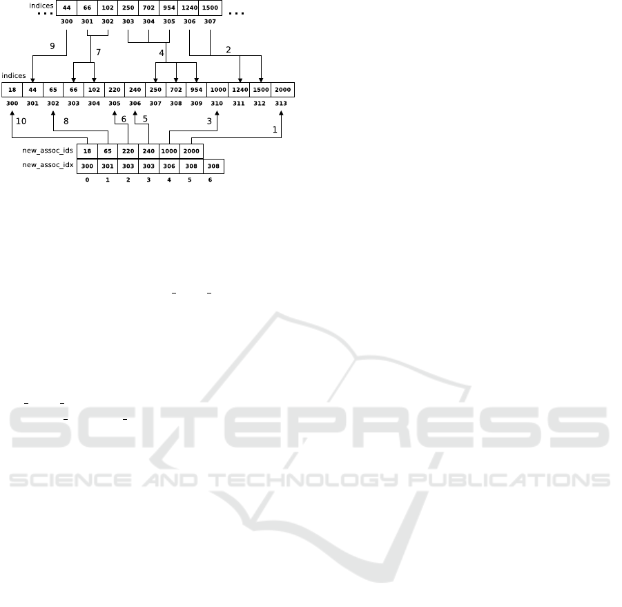
Figure 1: Inserting a cluster from a partition in the co-
association matrix. The arrows indicate to where the indices
are moved. The numbers indicate the order of the operation.
not the same, it means that old associations must be
moved as seen in the example. More specifically,
if the i-th element of the new assoc idx array, a, is
greater than the (i −1)-th element, b, then all the old
associations in the index interval [a, b[ are shifted to
the right by i positions. The i-th element will never
be smaller than the (i −1)-th because clusters are
sorted. Afterwards, or when two consecutive inser-
tion indices are the same, the (i −1)-th element of the
new assoc ids is inserted in the position indicated by
a pointer, o ptr. The o ptr pointer is initiazed with the
number of old associations plus the number of new
asociations and is decremented anytime an associa-
tion is moved or inserted. This showed to be roughly
twice as fast as using an implementation of quicksort.
3.4 EAC CSR Condensed
A further reduction of space complexity in the EAC
CSR scheme is possible by building only the up-
per triangular, since this completely describes the co-
association matrix. Thus, the amount of associations
decreases as one goes further down the matrix. In-
stead of pre-allocating the same amount of associa-
tions for each pattern, the pre-allocation follows the
same pattern of the number of associations, effec-
tively reducing the space complexity. The strategy
used was a linear one, where the first 5% of patterns
have access to 100% of the estimated maximum num-
ber of associations, the last pattern has access to 5%
of that value and the number available for the patterns
in between decreases linearly from 100% to 5%.
4 RECOVERY
We used Single-Link (SL) for the recovery of the fi-
nal partition. SL typically works over a pair-wise dis-
similarity matrix. An interesting property of SL is its
equivalence with a Minimum Spanning Tree (MST)
(Gower and Ross, 1969). In the context of EAC, the
edges of the MST are the co-associations between the
patterns and the vertices are the patterns themselves.
An MST contains all the information necessary to
build a SL dendrogram. One of the advantages of us-
ing an MST based clustering is that it processes only
non-zero values while a typical SL algorithm will pro-
cess all pair-wise proximities, even if they are null.
4.1 Kruskal’s Algorithm
Kruskal’s algorithm was used for computing the MST.
Kruskal (1956) described three constructs for finding
a MST, one of which is implemented efficiently in the
SciPy library (Jones et al., 2001): ”Among the edges
of G not yet chosen, choose the shortest edge which
does not form any loops with those edges already cho-
sen. Clearly the set of edges eventually chosen must
form a spanning tree of G, and in fact it forms a short-
est spanning tree.” This is done as many times as pos-
sible and if the graph G is connected, the algorithm
will stop before processing all edges when |V |− 1
edges are added to the MST, where V is the set of
edges. This implementation works on a CSR matrix.
One of the main steps of the implementation
is computing the order of the edges of the graph
without sorting the edges themselves, an operation
called argsort. The argsort operation on the ar-
ray [4, 5, 2, 1, 3] would yield [3, 2, 4, 0, 1] since the the
smallest element is at position 3 (starting from 0), the
second smalled at position 2, etc. This operation is
much less time intensive than computing the shortest
edge at each iteration. However, the total space used
is typically 8 times larger for EAC since the data type
of the weights uses only one byte and the number of
associations is very large, forcing the use of an 8 byte
integer for the argsort array. This motivated the stor-
age of the co-association matrix in disk and usage of
an external sorting algorithm.
4.2 External Memory Variant
The PyTables library (Alted et al., 2002), was used
for storing the co-association matrix in graph format,
performing the external sorting for the argsort oper-
ation and loading the graph in batches for process-
ing. This implementation starts by storing the CSR
graph to disk. However, instead of saving the in-
dptr array directly, it stores an expanded version of
the same length as the indices array, where the i-th
element contains the origin vertex (or row) of the i-
th edge. This way, a binary search for discovering
ICPRAM 2016 - International Conference on Pattern Recognition Applications and Methods
370
the origin vertex becomes unnecessary. Afterwards,
the argsort operation is performed by building a com-
pletely sorted index (CSI) of the data array of the CSR
matrix. It should be noted that the arrays themselves
are not sorted. Instead, the CSI allows for a fast index-
ing of the arrays in a sorted manner (according to the
order of the edges). The process of building the CSI
has a low main memory usage and can be disregarded
in comparison to the co-association matrix.
The SciPy implementation of Kruskal’s algorithm
was modified to work in batches. This was imple-
mented by making the data structures used in the
building of the MST persistent between iterations.
The new variant loads the graph in batches and in a
sorted manner, starting with the shortest edges. Each
batch is processed sequentially since the edges must
be processed in a sorted manner, which means there
is no possibility for parallelism. Typically, the batch
size is a very small fraction of the size of the edges,
so the total memory usage for building the MST is
overshadowed by the size of the co-association ma-
trix. As an example, for a 500 000 vertex graph the
SL-MST approach took 54.9 seconds while the exter-
nal memory approach took 2613.5 seconds - 2 orders
of magnitude higher.
5 RESULTS
Results presented here are originated from one of
three machines, that will be referred to as Alpha,
Bravo and Charlie. The main specifications of each
machine are as follows:
• Alpha: 4 GBs of main memory, a 2 core Intel i3-
2310M 2.1GHz and a NVIDIA GT520M;
• Bravo: 32 GBs of main memory, a 6 core Intel
i7-4930K 3.4GHz and a NVIDIA Quadro K600;
• Charlie: 32 GBs of main memory, a 4 core Intel
i7-4770K 3.5GHz and a NVIDIA K40c;
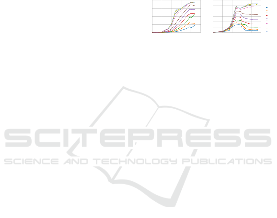
5.1 GPU Parallel K-Means
Both sequential and parallel versions of K-Means
were executed over a wide spectrum of datasets vary-
ing number of patterns, features and centroids. All
tests were executed on machine Charlie and the block
size was maintained constant at 512. The sequential
version used a single thread.
Observing Figures 2A and 2B, it is clear that the
number of patterns, features and clusters influence the
speed-up. For the simple case of 2 dimensions (Fig
2A), the speed-up increases with the number of pat-
terns. However, there is no speed-up when the overall
complexity of the datasets is low. As the complex-
ity of the problem increases (more centroids and pat-
terns), the speed-up also increases. The reason for this
is that the total amount of work increases linearly with
the number of clusters but is diluted by the number of
threads that can execute simultaneously.
10
8
6
4
2
0
Speed-up
10
2
10
6
10
5
10
4
10
3
Number of patterns
2
4
8
16
32
64
256
512
1024
2048
Number
of clusters
12
20
15
10
5
0
Speed-up
10
2
10
7
10
5
10
4
10
3
Number of patterns
(A) Datasets of 2 dimensions (B) Datasets of 200 dimensions
10
6
10
7
Figure 2: Speed-up of the labeling phase for datasets of (A)
2 dimensions and (B) 200 dimensions, when varying the
number of patterns and clusters. The dotted black line rep-
resents a speed-up of one.
For 200 dimensions (Fig. 2B), the speed-up in-
creased with both the number of patterns and clusters,
as previously. The speed-up obtained is lower than the
low dimensional case, which is consistent with liter-
ature (Zechner and Granitzer, 2009). The speed-up
decreased with an increase of the number of patterns
for a reduced number of clusters. We believe the rea-
son for this might be related to the implementation
itself. Our implementation does not use shared mem-
ory, which is fast.
5.2 Validation with Original
The results of the original version of EAC, imple-
mented in Matlab, are compared with those of the pro-
posed solution. Several small datasets, chosen from
the datasets used in (Lourenc¸o et al., 2010) and taken
from the UCI Machine Learning repository (Lichman,
2013), were processed by the two versions of EAC.
Both versions are processed from the same ensembles
since production is probabilistic, which guarantees
that the combination and recovery phases are equiv-
alent. All processing was done in machine Alpha. Ta-
ble 1 presents the difference between the accuracies
of the two versions. It is clear that the difference is
minimal, most likely due to the original version using
Matlab and the proposed using Python. Moreover, a
speed-up as low as 6 and as high as 200 was obtained
over the original version in the various steps.
5.3 Large Dataset Testing
The dataset used in the following results consists of a
mixture of 6 Gaussians, where 2 pairs are overlapped
and 1 pair is touching. This dataset was sampled into
smaller datasets to analyze different dataset sizes.
Efficient Evidence Accumulation Clustering for Large Datasets
371
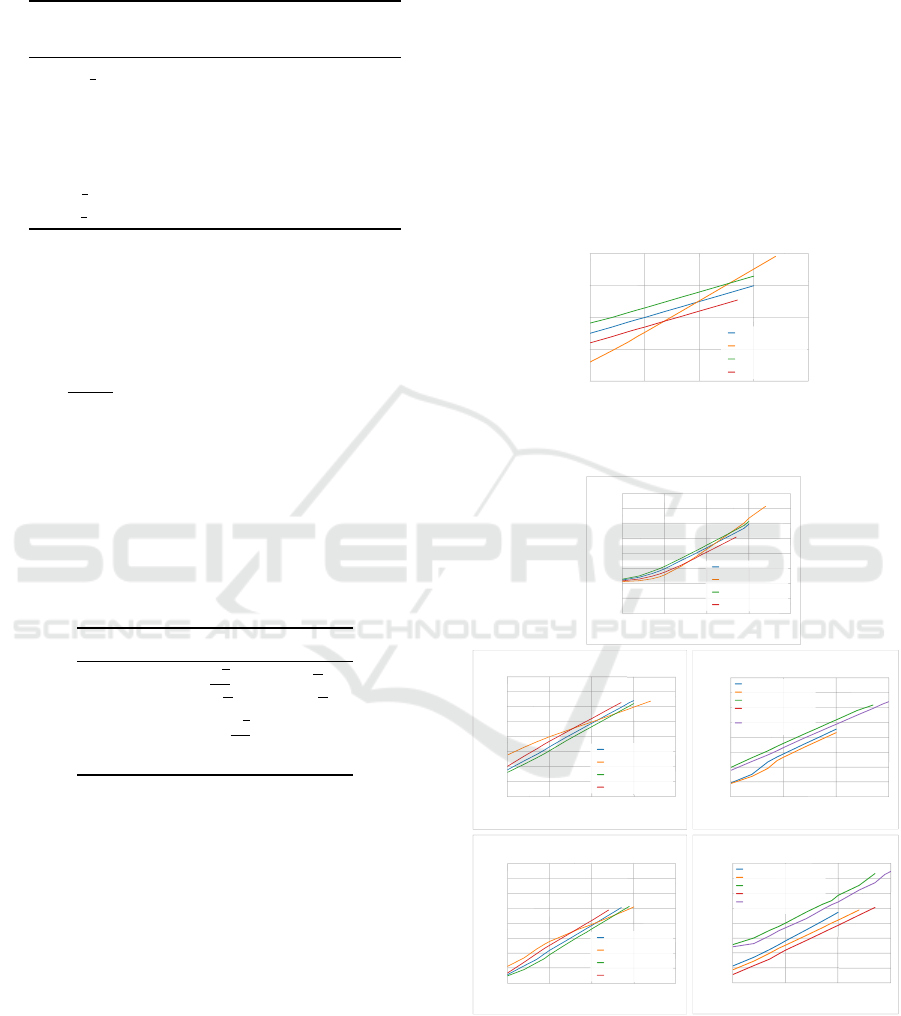
Table 1: Difference between accuracy of the two implemen-
tations of EAC, using the same ensemble. Accuracy was
measured using the H-index (Meila, 2003).
Number of clusters scheme
Dataset Fixed Lifetime
breast cancer 4.94e-06 2.82e-06
ionosphere 1.65e-06 1.45e-06
iris 3.33e-06 3.33e-06
isolet 1.03e-07 4.08e-07
optdigits 3.79e-06 1.48e-06
pima norm 4.16e-07 4.16e-07
wine norm 1.12e-07 1.91e-06
Several rules for computing the K
min
(see Table
2 for details), co-association matrix formats and ap-
proaches for the final clustering will be mentioned.
The co-association matrix formats are: full (for fully
allocated n ×n matrix), full condensed (for a fully al-
located
n(n−1)
2
array to build the upper triangular ma-
trix), sparse complete (for EAC CSR), sparse con-
densed const (for EAC CSR building only the upper
triangular matrix) and sparse condensed linear (for
EAC CSR condensed). The approaches for the fi-
nal clustering are SLINK (Sibson, 1973), SL-MST (for
using the Kruskal implementation in SciPy) and SL-
MST-Disk for a disk-based variant.
Table 2: Different rules for K
min
and K
max
. n is the number
of patterns and sk is the number of patterns per cluster.
Rule K
min
K
max
sqrt
√
n
2
√
n
2sqrt
√
n 2
√
n
sk=sqrt2 sk =
√
n
2
1.3K
min
sk=300 sk = 300 1.3K
min
A clustering ensemble was produced for each of
the smaller datasets and for each of the rules. From
each ensemble, co-association matrices were built. A
matrix format was not applicable if it could not fit in
main memory. The final clustering was done for each
of the matrix formats. The number of clusters was
chosen with the lifetime criteria (Fred and Jain, 2005).
SL-MST was not executed if its space complexity was
too big to fit in main memory. Furthermore, the com-
bination and recovery phases were repeated several
times, so as to make the influence of any background
process less salient. For big datasets, the execution
times are big enough that the influence of background
processes is negligible. All processing was done in
machine Bravo. Similar conclusions were drawn for
a dataset with separated Gaussians.
5.3.1 Execution Times
Execution times are related with the K
min
parameter,
whose evolution is presented in Fig. 3. Rules sqrt,
2sqrt and sk=sqrt2 never intersect but rule sk = 300
intersects the others, finishing with the highest K
min
.
Observing Fig. 4A, one can see that the same thing
happens to the production execution time associated
with the sk = 300 rule and the inverse happens to
the combination time (Fig. 4B). A higher K
min
means
more centroids for each K-Means run to compute, so
it is not surprising that the execution time for comput-
ing the ensemble increases as K
min
increases.
10
3
10
4
10
5
10
6
10
7
10
4
10
3
10
2
10
1
10
0
Number of samples
K
min
2sqrt
sk=300, th=30%
sk=sqrt2, th=30%
sqrt
Figure 3: Evolution of K
min
with the number of patterns for
different rules.
(A) Production of the clustering ensemble
10
5
10
4
10
3
10
2
10
1
10
0
10
-1
10
-2
10
-3
Time [s]
10
5
10
4
10
3
10
6
10
7
Number of samples
2sqrt
sk=300, th=30%
sk=sqrt2, th=30%
sqrt
10
6
10
5
10
4
10
3
Number of samples
10
5
10
4
10
3
10
2
10
1
10
0
10
-1
10
-2
10
-3
Time [s]
(C) Building the co-association matrix
with different matrix formats
full
full condensed
sparse complete
sparse condensed
const
sparse condensed
linear
(B) Building the co-association matrix
10
5
10
4
10
3
10
2
10
1
10
0
10
-1
10
-2
10
-3
Time [s]
10
5
10
4
10
3
10
6
10
7
Number of samples
2sqrt
sk=300, th=30%
sk=sqrt2, th=30%
sqrt
10
6
10
5
10
4
10
3
Number of samples
10
5
10
4
10
3
10
2
10
1
10
0
10
-1
10
-2
10
-3
Time [s]
(E) Comparison of three methods
for extraction
(D) Extraction with SL-MST
10
5
10
4
10
3
10
2
10
1
10
0
10
-1
10
-2
10
-3
Time [s]
10
5
10
4
10
3
10
6
10
7
Number of samples
2sqrt
sk=300, th=30%
sk=sqrt2, th=30%
sqrt
SLINK
SL-MST complete
SL-MST-Disk complete
SL-MST condensed
SL-MST-Disk
condensed
Figure 4: Execution time with different rules and variants
for: (A) production of the clustering ensemble; (B,C) build-
ing the co-association matrix; and (D,E) extraction of the
final partition with SL.
Fig. 4C shows the execution times on a longitu-
dinal study for optimized matrix formats. It is clear
that the sparse formats are significantly slower than
ICPRAM 2016 - International Conference on Pattern Recognition Applications and Methods
372
the fully allocated ones, specially for smaller datasets.
The full condensed usually takes around half the time
than the full, since it performs half the operations.
Idem for both sparse condensed compared to the
sparse complete. The discrepancy between the sparse
and full formats is due to the fact that the former needs
to do a binary search at each association update and
keep the internal sparse data structure sorted.
The clustering times of the different methods of
SL discussed previously (SLINK, SL-MST and SL-
MST-Disk) are presented in Figures 4D and 4E. As
expected, the SL-MST-Disk method is significantly
slower than any of the other methods, since it uses
the hard drive which has very slow access times
compared to main memory. SL-MST is faster than
SLINK, since it processes zero associations while SL-
MST takes advantage of a graph representation and
only processes the non-zero associations. In resem-
blance to what happened with combination times, the
condensed variants take roughly half the time as their
complete counterparts, since SL-MST and SL-MST-
Disk over condensed co-association matrices only
process half the number of associations. Although
this is not depicted, SLINK takes roughly the same
time for every rule, which means K
min
has no influ-
ence because SLINK processes the whole matrix, re-
gardless of its association sparsity. The same rationale
can be applied to SL-MST, where different rules can
influence execution times, since they change the to-
tal number of associations. As with the combination
phase, the sk=300 rule started with the greatest exe-
cution time and decreased as the number of patterns
increased until it was the fastest.
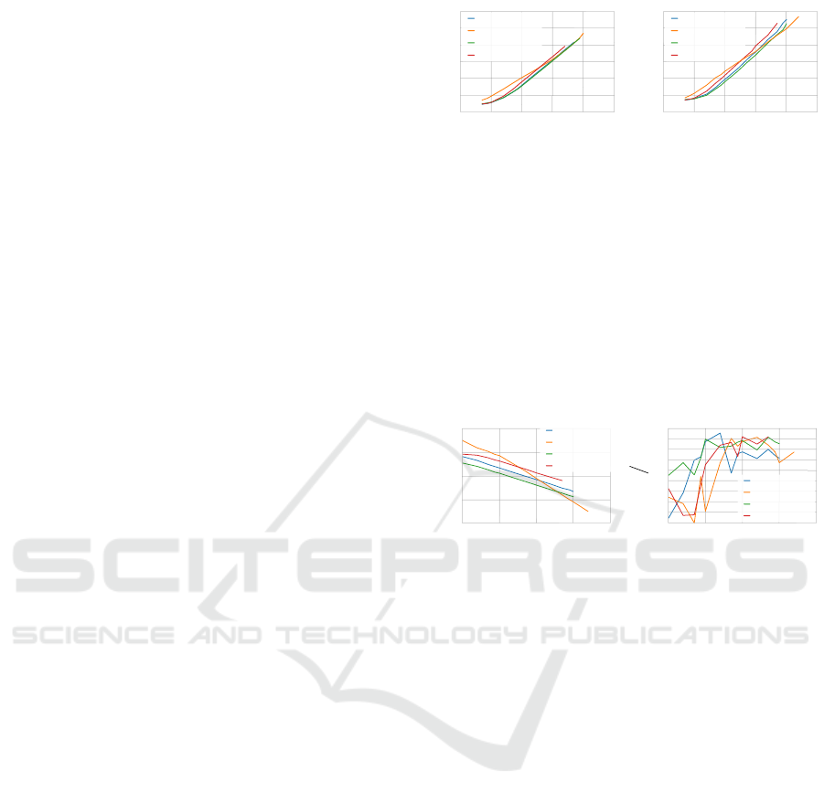
The total execution times presented in Fig. 5 are
for the sparse condensed linear format but the oth-
ers follow the same pattern. When using the SL-MST
method in the recovery phase, the execution time for
three of the rules do not differ much. This is due to
a balancing between a slow down of the production
phase and a speed up of the combination and recovery
phases as K
min
increases at a higher rate for sk = 300
than for other rules. This is not observed for the sqrt
rule as K
min
is always low enough that the total time
is always dominated by the combination and recov-
ery phases. However, when using the SL-MST-Disk
method, the total time is dominated by the recovery
phase. This is clear, since the results in Fig. 5B fol-
low the tendency presented in Fig. 4D.
5.3.2 Association Density
The aforementioned sparse nature of EAC is clear in
Fig. 6A. This figure shows the association density, i.e.
number of associations relative to the n
2
associations
in a full matrix. The full condensed has, roughly, a
10
6
10
5
10
4
10
3
Number of samples
10
5
10
4
10
3
10
2
10
1
10
0
10
-1
Time [s]
(A) Recovery phase with SL-MST (B) Recovery phase with SL-MST-Disk
10
7
10
2
10
6
10
5
10
4
10
3
Number of samples
10
7
10
2
10
5
10
4
10
3
10
2
10
1
10
0
10
-1
Time [s]
2sqrt
sk=300, th=30%
sk=sqrt2, th=30%
sqrt
2sqrt
sk=300, th=30%
sk=sqrt2, th=30%
sqrt
Figure 5: Execution times for all phases combined, using
(A) SL-MST and (B) SL-MST-Disk in the recovery phase.
constant density of 50%. Idem for all sparse formats,
as long as no associations are discarded. The den-
sity should decrease as the number of patterns of the
dataset increases, since the full matrix grows quadrat-
ically. Besides, it would be expected that the same as-
sociations would be grouped together more frequently
in partitions and make previous connections stronger
instead of creating new ones, if the relationship be-
tween the number of patterns and K
min
is constant.
10
6
10
5
10
4
10
3
Number of samples
10
0
10
-1
10
-2
10
-3
Density
1.0
(B) Relationship between max. number
associations and biggest cluster size
10
7
10
6
10
5
10
4
10
3
Number of samples
10
7
10
-4
1.4
1.8
2.2
2.6
(A) Density of associations relative
to full matrix
2sqrt
sk=300, th=30%
sk=sqrt2, th=30%
sqrt
2sqrt
sk=300, th=30%
sk=sqrt2, th=30%
sqrt
max number biggest
associations / cluster size
Figure 6: (A) Density of associations relative to the full co-
association matrix, which hold n
2
associations. (B) Maxi-
mum number of associations of any pattern divided by the
number of patterns in the biggest cluster of the ensemble.
Predicting the number of associations is useful for
designing combination schemes that are both memory
and speed efficient. Fig. 6B presents the ratio between
the biggest cluster size and the maximum number of
associations of any pattern. This ratio increases with
the number of patterns, but never exceeds 3. However,
the number of features of the used datasets is small. It
might be the case that this ratio would increase with
the number of features, since there would be more de-
grees where the clusters might include other neigh-
bors. Thus, further studies with a wider spectrum of
datasets should yield more enlightening conclusions.
5.3.3 Space Complexity
The allocated space for the space formats is based on
a prediction that uses the biggest cluster size of the
ensemble. This allocated space is usually more than
what is necessary to store the total number of associa-
tions, to keep a safety margin. Furthermore, the CSR
format, on which the EAC CSR strategy is based, re-
quires an array of the same size of the predicted num-
ber of associations. Still, the allocated number of as-
sociations becomes a very small fraction compared
Efficient Evidence Accumulation Clustering for Large Datasets
373

to the full matrix as the dataset complexity increases,
which is the typical case for using a sparse format.
The actual memory used is presented in Fig. 7. The
data types influence significantly the required mem-
ory. The associations can be stored in a single byte,
since the number of partitions is usually less than 255.
This means that the memory used by the fully allo-
cated formats is n
2
and
n(n−1)
2
Bytes for the complete
and condensed versions, respectively. In the sparse
formats, the values of the associations are also stored
in an array of unsigned integers of 1 Byte. However,
an array of integers of 4 bytes of the same size must
also be kept to keep track of the destination pattern
each association belongs to. One other array of inte-
gers of 8 bytes is kept but it is negligible compared to
the other two arrays. The impact of the data types can
be seen for smaller datasets where the total memory
used is actually significantly higher than that of the
full matrix. It should be noted that this discrepancy is
not as high for other rules as for sk = 300. Still, the
sparse formats, and in particular the condensed sparse
format, are preferred since the memory used for large
datasets is a small fraction of what would be neces-
sary if using any of the fully allocated formats.
10
3
10
4
10
5
10
6
10
7
10
2
10
1
10
0
10
-1
10
-2
Number of samples
Density
full
full condensed
sparse complete
sparse condensed const
sparse condensed linear
10
-3
Figure 7: Memory used relative to the full n
2
matrix. The
sparse complete and sparse condensed const curves are
overlapped.
6 CONCLUSIONS
The main goal of scaling the EAC method for larger
datasets than was previously possible was achieved.
The EAC method is composed by three steps and, to
scale the whole method, each step was optimized sep-
arately. In the process, EAC was also optimized for
smaller datasets. In essence, the main contributions
to the EAC method, by step, were the GPU parallel
K-Means, the EAC CSR strategy and the SL-MST-
Disk. New rules for K
min
were tested and the effects
that these rules have on other properties of EAC were
studied. Together, these contributions allow for the
application of EAC to datasets whose complexity was
not handled by the original implementation.
Further work involves a thorough evaluation in
real world problems. Additional work may include
further optimization of the Parallel GPU K-means by
using shared memory and a better sorting of the co-
association graph in SL-MST-Disk.
ACKNOWLEDGEMENTS
This work was supported by the Portuguese Founda-
tion for Science and Technology, scholarship num-
ber SFRH/BPD/103127/2014, and grant PTDC/EEI-
SII/7092/2014.
REFERENCES
Alted, F., Vilata, I., and Others (2002). PyTables: Hierar-
chical Datasets in Python.
Fred, A. (2001). Finding consistent clusters in data parti-
tions. Multiple classifier systems, pages 309–318.
Fred, A. N. L. and Jain, A. K. (2005). Combining multiple
clusterings using evidence accumulation. IEEE Trans.
Pattern Anal. Mach. Intell., 27(6):835–850.
Gower, J. C. and Ross, G. J. S. (1969). Minimum Spanning
Trees and Single Linkage Cluster Analysis. Journal
of the Royal Statistical Society, 18(1):54–64.
Jain, A. K. (2010). Data clustering: 50 years beyond K-
means. Pattern Recognition Letters, 31(8):651–666.
Jones, E., Oliphant, T., Peterson, P., and Others (2001).
SciPy: Open source scientific tools for Python.
Lichman, M. (2013). {UCI} Machine Learning Repository.
Lindholm, E., Nickolls, J., Oberman, S., and Montrym, J.
(2008). Nvidia tesla: A unified graphics and comput-
ing architecture. IEEE micro, (2):39–55.
Lourenc¸o, A., Fred, A. L. N., and Jain, A. K. (2010). On the
scalability of evidence accumulation clustering. Proc.
- Int. Conf. on Pattern Recognition, 0:782–785.
Meila, M. (2003). Comparing clusterings by the variation
of information. Learning theory and Kernel machines,
Springer:173–187.
Sibson, R. (1973). SLINK: an optimally efficient algo-
rithm for the single-link cluster method. The Com-
puter Journal, 16(1):30–34.
Sirotkovi, J., Dujmi, H., and Papi, V. (2012). K-means im-
age segmentation on massively parallel GPU architec-
ture. In MIPRO 2012, pages 489–494.
Strehl, A. and Ghosh, J. (2002). Cluster Ensembles – A
Knowledge Reuse Framework for Combining Multi-
ple Partitions. J. Mach. Learn. Res., 3:583–617.
Zechner, M. and Granitzer, M. (2009). Accelerating k-
means on the graphics processor via CUDA. In IN-
TENSIVE 2009, pages 7–15.
ICPRAM 2016 - International Conference on Pattern Recognition Applications and Methods
374
