Bayesian Inference in Dynamic Domains using Logical OR Gates
Rik Claessens
1,2
, Alta de Waal
3
, Pieter de Villiers
3,4
, Ate Penders
2,5
, Gregor Pavlin
2,6
and Karl Tuyls
1,5
1
University of Liverpool, Liverpool, U.K.
2
Thales Research & Technology, Delft, the Netherlands
3
University of Pretoria, Pretoria, South Africa
4
Council for Scientific and Industrial Research, Pretoria, South Africa
5
Delft University of Technology, Delft, The Netherlands
6
University of Amsterdam, Amsterdam, The Netherlands
Keywords:
Artificial Intelligence and Decision Support Systems, Multi-agent Systems, Strategic Decision Support
Systems.
Abstract:
The range of applications that require processing of temporally and spatially distributed sensory data is
expanding. Common challenges in domains with these characteristics are sound reasoning about uncertain
phenomena and coping with the dynamic nature of processes that influence these phenomena. To address
these challenges we propose the use of causal Bayesian Networks for probabilistic reasoning and introduce
the Logical OR gate in order to combine them with dynamic processes estimated by arbitrary Markov
processes. To illustrate the genericness of the proposed approach, we apply it in a wildlife protection use
case. Furthermore we show that the resulting model supports modularization of computations, which allows
for efficient decentralized processing.
1 INTRODUCTION
Recent advances in sensory, computing and commu-
nication technology have facilitated a new class of
decision support applications that exploit rich and
heterogeneous data to estimate the phenomena rele-
vant for decision making and control. Such applica-
tions are gaining importance in various domains, such
as security, smart homes, Internet of Things (IoT),
etc. For example, imminent threats in security appli-
cations must be identified based on various sensory
clues and intelligence. Similarly, in the domain of
elderly care, heterogeneous data obtained via IoT de-
vices can provide clues about anomalies correspond-
ing to potentially dangerous states of an elderly per-
son.
While the potential of this range of applications
is huge, there are multiple challenges associated with
correct and tractable processing of the correlated
data, stemming from disparate sources (e.g. sensors,
human observers, databases, social media, etc.) and
collected at different locations and points in time.
Such processing depends on domain models that
describe correlations between the different data types
and the inference algorithms that use such models to
draw conclusions about the phenomena of interest. In
the targeted domains, the modelling and inference are
not trivial, however. These domains are characterized
through many types of correlated phenomena and
dynamic processes. The resulting domain models
may contain many variables and the dynamics must
be appropriately considered.
Without the loss of generality, we will use a run-
ning example from wildlife protection focusing on the
prevention of rhino poaching to illustrate the chal-
lenges and solutions (Figure 1). As the resources for
observing, patrolling or intervening in such environ-
ments are limited and the areas that need to be pro-
tected vast, a decision support system using different
types of data is needed to help with the assessment
of potentially critical locations where the poaching
could take place. The threat depends on many differ-
ent factors, such as environmental conditions as well
as the presence of the rhinos, rangers and the poach-
ers. Moreover, the observations of potential poach-
ers are often sparse and uncertain. The same is true
for the location of rhinos. Consequently, situation as-
sessment requires collection of many different types
134
Claessens, R., Waal, A., Villiers, P., Penders, A., Pavlin, G. and Tuyls, K.
Bayesian Inference in Dynamic Domains using Logical OR Gates.
In Proceedings of the 18th International Conference on Enterprise Information Systems (ICEIS 2016) - Volume 2, pages 134-142
ISBN: 978-989-758-187-8
Copyright
c
 2016 by SCITEPRESS – Science and Technology Publications, Lda. All rights reserved

of data at different locations and points in time and
reasoning about the observed patterns. As data col-
lection and reasoning in such settings typically ex-
ceed the capabilities of human operators (D
¨
orner and
Schaub, 1994), an automated information fusion sys-
tem is used.
(a) (b) (c)
Figure 1: An overview of a threat assessment system in
the Kruger and Limpopo National Parks in South Africa.
Figure 1(a) shows poacher and rhino locations (icons)
and their tracks (dashed lines). A continuous heat-map
visualizing high-risk zones and a discretized grid-based
heat-map are shown in Figure 1(b) and 1(c) respectively.
This use case illustrates a class of applications that
require inference combining (i) dynamic models de-
scribing the evolution of processes over space and
time and (ii) location bound models that describe re-
lations between different factors at a specific location.
This paper addresses multiple challenges associ-
ated with such analysis. Firstly, the dynamic and loca-
tion bound models have to be combined in a theoreti-
cally sound and efficient manner. For this we propose
the use of causal Bayesian Networks (BN) and so-
called Logical OR gates, that allow creation of com-
plex causal probabilistic domain models. Secondly,
we show that the presented Bayesian approach fa-
cilitates modularization of models and inference pro-
cesses, that can be computed in a distributed fashion.
The paper is structured as follows: Section 2
discusses related work on Bayesian Networks. In
Section 3, we introduce the relevant probabilistic
models and propose the use of Logical OR gates for
combining dynamic elements with a static situation
assessment BN. Section 4 discusses how the proposed
methods can be applied in a rhino poaching domain.
Afterwards we explain how the use of Logical OR
gates results in a modular probabilistic network.
Finally, we draw some conclusions and steps for
future research in the last section.
2 RELATED WORK
Related work mainly comes from two research areas,
i.e., Bayesian networks (specifically for environmen-
tal modelling) and distributed inference systems.
Bayesian networks (BNs) are well established
method supporting systematic exploitation of corre-
lated data and are often used as a modelling tool
for environmental modelling with a wide range of
case studies to be found in literature (Pearl, 1988;
Johnson et al., 2010; Pullar and Phan, 2007; Borsuk
et al., 2004; Borsuk et al., 2006). Furthermore, BNs
are ideal to combine knowledge from diverse disci-
plines and sources (D
¨
uspohl et al., 2012) and hence
Bayesian Network (BN) models can be learned from
data and/or constructed with involvement of domain
experts. This is often referred to as ‘participatory
modelling’ (Bromley et al., 2005).
An important challenge of an inference system is
to cope with large quantities of heterogeneous infor-
mation that becomes available dynamically, at run-
time. The inference systems must be adapted at
runtime, which requires modular approaches, where
loosely coupled inference modules collaboratively
solve an assessment problem through message pass-
ing. There exist multiple approaches to achieve sound
inference in modular systems, which perform exact
inference with the help of secondary inference struc-
tures, such as junction trees, linked junction forests
and spanning multiple processing modules (Xiang,
2002; Paskin and Guestrin, 2004). Compilation of
such structures, however, requires expensive process-
ing and massive messaging, which in turn can be
impractical if constellations of information sources
change rapidly. In this paper we use an alternative
modularization approach to exact inference (Pavlin
et al., 2010; de Oude and Pavlin, 2009), where com-
pilation of secondary structures is avoided.
3 PROBABILISTIC MODELS
Models describing the correlations between the obser-
vations and hidden phenomena of interest are indis-
pensable for sound inference. The various observa-
tions collected by the fusion system can be viewed as
outcomes of a system of interrelated causal processes.
Therefore it is reasonable to use Bayesian Networks
and Hidden Markov Model approaches, as they can
efficiently and systematically describe the dependen-
cies between the phenomena. In the targeted domains,
however, complex models are required, consisting of
many variables and relations. Monolithic approaches
to modelling and inference cannot cope with such
complexity. However, it turns out that the overall do-
main models can be viewed as a composition of two
types of models:
Bayesian Inference in Dynamic Domains using Logical OR Gates
135

• Location Bound Model (LBM), that describes the
relations between the various factors influencing
the phenomena of interest at a specific location.
Such a model correlates the phenomena of interest
with the presence of one or multiple dynamic
objects at the respective location and various
environmental phenomena.
• Models of dynamic processes that describe the
relations between states corresponding to multiple
locations and different points in time, such as
tracked objects.
In the presented approach, we assume that the area
of interest is represented by a grid, where each cell
corresponds to a location labelled a
k
(Figure 1(a)).
Each location is associated with an LBM that is used
for the estimation of the states of hidden phenomena
of interest at a certain location a
k
at time t.
The two types of reasoning mentioned above re-
quire adequate representations and inference algo-
rithms. Furthermore, a correct method that allows
combining the LBMs with the dynamic models is re-
quired. These aspects are discussed in the following
subsections.
3.1 Location Bound Models
An LBM describes correlations between the observ-
able phenomena/events at a
k
and the hidden phenom-
ena that influence the observable events.
In the presented approach, location bound models
(LBMs) are represented through causal BNs (Pearl,
1988). A BN is defined as a tuple hG, Pi, where G =
hV , Ei is a Directed Acyclic Graph (DAG) defining a
domain V = {V
1
, . . . , V
n
} and a set of directed edges
hV
i
, V
j
i ∈ E over the domain. The Joint Probability
Distribution (JPD) P(V ) over the domain V is de-
fined as P(V ) =
∏
V
P(V
i
|π(V
i
)), where P(V
i
|π(V
i
))
is the conditional probability distribution for node V
i
given its parents π(V
i
), which can be represented by a
Conditional Probability Table (CPT). BNs allow ef-
ficient representation of the states of heterogeneous
phenomena and describe causal relations between
these phenomena. Moreover, they support mathemat-
ically sound and efficient inference algorithms.
3.2 Dynamic Models
Dynamic models capture correlations between spa-
tially and temporally distributed phenomena and
events associated with evolving processes, such as
moving objects. These evolutionary processes can be
represented with the help of Hidden Markov Models
or their generalization, Dynamic Bayesian Networks
(DBNs) (Thrun et al., 2005). In these approaches the
inference is carried out on models that are expanded
with identically structured slices over time (Figure
2). Such inference is called tracking if we estimate
the states of a moving object. In this paper we as-
sume a common technique for approximate inference
in such models, namely Particle Filters (Gustafsson
et al., 2002). The Particle Filter (PF)-algorithm makes
use of a set of particles, representing possible loca-
tions of the entity that is being tracked. The distri-
bution or spread of the set of particles gives a mea-
sure for the uncertainty about the target’s true loca-
tion. The continuous probability distribution that a
PF-algorithm approximates is given by the posterior
probability distribution over the state of interest, in
this case the location x
t
of target j: P(x
t
|Z
j
1:t
), where
Z
j
1:t
denotes the sequence of all observations of the
tracked object. .
x
0
z
0
x
1
z
1
· · ·
x
t−1
z
t−1
x
t
z
t
T
j
k,t
Figure 2: The structure of the DBN that is approximated by
a PF-based tracking algorithm. The dashed edge represents
the function in(x
i
t
, a
k
) from Equation 2.
We introduce a binary variable, T
j
k,t
, whose states
represent the presence of an individual or a group
of tracked object(s) (indexed by j) being present in
area a
k
at time t. The posterior probability of a T
j
k,t
is in principle an integral of the probability distribu-
tion, representing the spatial distribution of tracked
objects, over area a
k
. However, since the set of par-
ticles approximates a continuous probability distribu-
tion with a set of discrete particles, we approximate
this integral with the number of particles that are in-
side a
k
, divided by the total number of particles N:
P(T
j
k,t
= true|Z
j
1:t
) =
Z
a
k
P(x
t
|Z
j
1:t
)dx
≈
1
N
∑
i
in(x
i
t
, a
k
), (1)
where the function in(x
i
t
, a
k
) is defined as:
in(x
i
t
, a
k
) =
(
1, if x
i
t
is inside area a
k
0, otherwise
. (2)
3.3 Combining Tracking and Location
Bound Models
The question is, how the DBN shown in Figure 2 can
be combined with an LBM in a mathematically sound
ICEIS 2016 - 18th International Conference on Enterprise Information Systems
136

way. An additional challenge is that multiple dynamic
objects could be present at a specific location. Con-
sequently, dependent on the situation, the LBM might
have to be combined with multiple DBNs, each es-
timating the whereabouts of a different dynamic ob-
ject. Thus, the estimation of the hidden phenomena
of interest depends on evolving domain models. The
solution is achieved in a number of steps.
First we consider the variable whose states are
influenced by the outputs of tracking processes. As
we assume that in an LBM there exists a “Track
Present” (T P), a binary variable representing the
presence of any object at the location associated with
that LBM. In the discretized setting, the distribution
over the binary variable is computed for a specific
location and time, i.e. TP
k,t
represents the situation
that any number of dynamic objects is present in
area a
k
at time t. Consequently, at any moment in
time at any location, a varying number of tracks may
influence the LBM that is performing the inference
for that area.
Figure 3 shows the structure of the part of the BN
described above. There is an edge from every T
j
k,t
variable (representing a single track) converging to
TP
k,t
. The dynamic nature of the tracks means that
the structure of the BN changes as tracks enter and
leave an area.
T P
k,t
T
1
k,t
T
2
k,t
· · ·
T
n
k,t
Figure 3: The BN structure of a connection between
tracking processes T
j
k,t
and the BN variable TP
k,t
they
influence.
The CPT of the variable TP
k,t
is determined by
the set of incoming edges, i.e. the set of tracks that
have an influence in an area a
k
. In this paper, the
CPT has a physical interpretation. For each area
defined in the system, the tracked target is either
present (with probability 1) or not present at all
(thus, a probability of 0 for being present). This
interpretation results in a straightforward definition
of the entries in the CPT. Namely, the entries in
the columns P(TP
k,t
|T
1
k,t
, . . . , T
n
k,t
), for which ∃ T
j
k,t
∈
{T
1
k,t
, . . . , T
n
k,t
}, s.t. T
j
k,t
= true are set as [
1 0
]
T
.
This includes all columns in the CPT, except one.
This is the column, for which ∀ T
j
k,t
∈ {T
1
k,t
, . . . , T
n
k,t
},
T
j
k,t
= f alse. This assignment of random variables
represents the situation where no tracked objects are
present in a specific area. Therefore, we set this
column as [
0 1
]
T
.
Table 1: A schematic overview of the CPT of the variable
TP
k,t
, i.e. P(TP
k,t
|T
1,k,t
, . . . , T
j,k,t
).
T
n
k,t
t f
.
.
.
.
.
. .
.
.
T
2
k,t
t f ·· · f
T
1
k,t
t f t f ··· ··· t f
TP
k,t
t 1 1 1 1
·· ·
1 0
f 0 0 0 0 0 1
The resulting CPT is shown in Table 1 and is
called a logical OR gate. Although the entries in the
CPT consist only of 0s and 1s, uncertainty about a
target’s true location is introduced by the computation
of the prior probability distribution of each T
j
k,t
node.
The logical OR gate can be used to integrate
the LBM with dynamic models. This integration
results in an overall more complex, but because of
the presented approach easily tractable BN. The
next section illustrates a BN in which tracks are
incorporated.
3.4 Posteriors of Tracking Modules
The CPT from Table 1 is used to compute the belief
over the tracked entity being present in area a
k
. This
marginalization is given by:
P(TP
k,t
= true|Z
1:t
)
=
∑
T
1
k,t
. . .
∑
T
j
k,t
h
P(TP
k,t
= true|T
1
k,t
, . . . , T
j
k,t
)
·
∏
j
P(T
j
k,t
|Z
j
1:t
)
i
. (3)
This marginalization is the product of probabili-
ties of each permutation of tracked objects that are
present in area a
k
. By exploiting the structure of the
CPT however, there is a much faster way to compute
the posterior. Namely, it is possible to compute the
belief that a tracked entity is present in area a
k
as the
product of the probabilities of each tracked object be-
ing absent in the area,
∏
j

1 − P(T
j
k,t
= true|Z
j
1:t
)

.
We show that this is equivalent to the marginalization
for TP
k,t
= true over all T
j
k,t
variables.
We will exploit the characteristics of a binary
variable:
P(TP
k,t
= true
k,t
|Z
1:t
) = 1−P(TP
k,t
= f alse|Z
1:t
)
(4)
From Table 1, it it is clear that
P(TP
k,t
= f alse|T
1
k,t
, . . . , T
j
k,t
) only resolves to 1, if
Bayesian Inference in Dynamic Domains using Logical OR Gates
137

and only if ∀ T
j
k,t
∈ {T
1
k,t
, . . . , T
n
k,t
}, T
j
k,t
= f alse. We
combine Equations 3 and 4:
P(TP
k,t
= f alse|Z
1:t
)
=
∑
T
1
k,t
. . .
∑
T
j
k,t
h
P(TP
k,t
= f alse|T
1
k,t
, . . . , T
j
k,t
)
·
∏
j
P(T
j
k,t
|Z
j
1:t
)
i
(5)
The marginalization in Equation 5 is a sum over
zero-valued products, except the case where all T
j
k
variables have value T
j
k
= f alse. Because of this we
are able to simplify Equation 5 to:
P(TP
k,t
= f alse|Z
1:t
) =
∏
j
P(T
j
k,t
= f alse|Z
j
1:t
) (6)
As we are interested in the posterior for TP
k,t
=
true, we subtract this value from 1. As a final step,
by combining Equations 3, 4 and 5 and observing
that, by definition P(T
j
k,t
= f alse|Z
1:t
) = 1 − P(T
j
k,t
=
true|Z
1:t
), the computation of the posterior of TP
k,t
=
true can be simplified as:
P(TP
k,t
= true|Z
1:t
)
k
= 1 −
∏
j

1 − P(T
j
k,t
= true|Z
j
1:t
)

. (7)
By using the models and equations described
above it is possible to incorporate tracking informa-
tion into an LBM, without the need of changing the
model at runtime.
4 APPLICATION: RHINO
POACHING
In this section we will apply the in the previous
sections explained methods in a present-day security
setting, rhino poaching in the Kruger Park, South
Africa.
4.1 Bayesian Threat Assessment
An example of a BN that describes correlations
between poaching events was introduced by (Koen
et al., 2014). For the sake of simplicity, we use a
derived BN, shown in Figure 4. To make the notation
of variables more compact, we abbreviate all variable
names to the bold and underlined parts in Figure 4
in the remaining part of this paper. Furthermore, we
use superscripts R, P and Ra for variables relating to
rhinos, poachers and rangers respectively.
Poaching Event
Poaching Report
Vulnerability
Moon
Weather
Time Of Day
Rhino Present
Poacher Present
Ranger Present
Figure 4: A BN describing phenomena that influence the
likelihood of a poaching event.
The BN in Figure 4 corresponds to the following
joint probability density (JPD) factorization:
JPD = P(PE|Vu, PP, RP, RaP)P(PR|PE)
· P(Vu|Mo, We, T )P(Mo)P(We)P(T )
· P(PP)P(RP)P(RaP). (8)
A separate instance of this model is used for each
area, i.e. a cell, represented in the grid-based map
shown in Figure 1(c). Each model correlates different
types of observations obtained in the respective area
a
k
.
There are a number of entities of importance for
which information should be gathered, such as the
poachers and rhinos in Figure 1(a).
The states of nodes labelled Poacher Present
and Rhino Present represent dynamic objects, as de-
scribed by the variable “Track Present” (T P) in the
previous section. However, the events corresponding
to the states of these variables are not observed di-
rectly. The states of rhinos and poachers are typically
estimated with the help of tracking processes based
on filters that correlate spatio-temporal observations.
As described before, the dynamic nature of the
tracks would require to modify the structure of the
BN dynamically at runtime. However, considering
the size of the area in which the system will be
deployed, the number of areas and tracks might
grow too large in order to perform computations
of inference algorithms such as the sum-product
algorithm efficiently. To avoid this computationally
expensive task, we incorporate logical OR gates in the
BN from Figure 4.
The JPD of the network shown in Figure 5 then
resolves to:
JPD
k,t
= P(PE|Vu, PP, RP, RaP)P(PR|PE)
· P(Vu|Mo, We, T )P(Mo)P(We)P(T )
· P(PP|T
1,P
k,t
, . . . , T
j,P
k,t
)
∏
j
P(T
j,P
k,t
|Z
P
1:t
)
· P(RP|T
1,R
k,t
, . . . , T
l,R
k,t
)
∏
l
P(T
l,R
k,t
|Z
R
1:t
)
· P(RaP|T
1,Ra
k,t
, . . . , T
m,Ra
k,t
). (9)
ICEIS 2016 - 18th International Conference on Enterprise Information Systems
138

PE
Vu
T
Mo
We
PP
T
P
1,k,t
x
t
x
t−1
· · ·
x
0
z
t
z
t−1
z
0
T
P
1
· · ·
· · ·
T
P
j,k,t
x
t
x
t−1
· · ·
x
0
z
t
z
t−1
z
0
T
P
j
RP
T
R
1,k,t
x
t
x
t−1
· · ·
x
0
z
t
z
t−1
z
0
T
R
1
· · ·
· · ·
T
R
l,k,t
x
t
x
t−1
· · ·
x
0
z
t
z
t−1
z
0
T
R
l
RaP
T
1
Ra
T
2
Ra
· · ·
T
n
Ra
PR
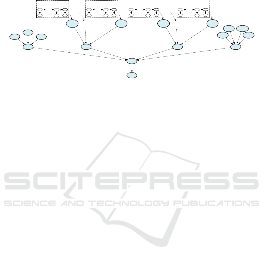
Figure 5: A BN using logical OR gates for inserting poacher, rhino and ranger tracks. Superscripts R, P and Ra denote
variables for rhinos, poachers and rangers respectively.
By using the simplification from Equation 7, the
posterior probability of the variable Poaching Event
based on the BN from Figure 5 (Equation 9), is
given by Equation 10 (in which η is the normalization
factor).
P(PE
k,t
= true|Z
P
1:t
, Z
R
1:t
, E
P
1:t
, E
R
1:t
, E
Vu
1:t
, X
Ra
1:t
)
k
= η
∑
TP
∑
RP
∑
Vu
∑
Ra

P(PE
k,t
= true|Vu
k,t
, TP
k,t
, RP
k,t
, RaP
k,t
)
· P(PR
k,t
|PE
k,t
= true)
·
∑
We
h
P(Vu
k,t
|Mo
k,t
, We
k,t
, T
k,t
)
· P(Mo
k,t
)P(We
k,t
)P(T
k,t
)
i
·
h
1 −
∏
j

1 − P(T
j,P
k,t
= true|Z
j,P
1:t
)

i
·
h
1 −
∏
l

1 − P(T
l,R
k,t
= true|Z
l,R
1:t
)

i
·
h
1 −
∏
m

1 − P(T
m,Ra
k,t
= true)

i

(10)
5 DISTRIBUTED INFERENCE
In this section we discuss how the previously intro-
duced domain models can be split up into modules
that allow distributed computation. The notion of
Markov boundaries is used to show that this type of
distributed computation results in sound inference.
Furthermore, the different types of agents that con-
stitute this Multi-Agent System (MAS) are discussed
as well as the complexity of the overall system.
By using logical OR gates for combining tracking
processes and the LBMs, we obtain a system that
is equivalent to a BN that describes the overall
situation (Figure 5). This model captures correlations
between disparate observations that are relevant for
the estimation of the likelihood of a poaching event,
such as the observations of poachers or rhinos as well
as the phenomena that define the context of the event
and further a priori knowledge.
This model is a basis for the computation of the
probability of poaching which corresponds to the
evaluation of Equation 10.
5.1 Model Decomposition
The fact that we can write the correlations in the form
of a BN reveals important properties of the overall
joint distribution over all variables in the BN. Namely,
not all variables are directly dependent, which allows
efficient modelling and inference.
We exploit the concept of d-separation to partition
the BN shown in Figure 5 into smaller BN fragments
according to the design rules presented in (Pavlin
et al., 2010). We obtain fragment Ψ
LBM
k
(denoted by
the coloured nodes in figure 5) and tracker fragments
Ψ
j,P
and Ψ
l,R
that correspond to the network shown in
Figure 2. Each fragment Ψ
i
is a BN defined over a set
of variables V
i
∈ V , where V denotes the variables
from the original BN. In each fragment Ψ
i
we can
identify a Markov Boundary (MB
i
), a set of variables
X
i
∈ V
i
. If all variables in MB
i
are instantiated with
hard evidence, then the inference over other variables
V
i
in Ψ
i
is rendered independent of other variables in
the original BN (Pearl, 1988). In the used fragments
we can identify the following Markov Boundaries:
• Each Ψ
LBM
k
is associated with
MB
LBM
k,t
= {[T
j,P
k,t
], [T
l,R
k,t
], [T
m,Ra
k,t
]}
• Each Ψ
j,P
is associated with
MB
P
j,k,t
= {T
j,P
k,t
}
• Each Ψ
l,R
is associated with
MB
R
l,k,t
= {T
l,R
k,t
}
Bayesian Inference in Dynamic Domains using Logical OR Gates
139

Note, the rectangular brackets [ ] denote multiple
variables associated with different tracker fragments
contributing beliefs to the LBM at a
k
. It turns out
that in such domains (i) the intersection of MB of
Ψ
LBM
k
and the MB of any track fragment contains at
most one uninstantiated variable (T
j,P
k,t
or T
l,R
k,t
) and
(ii) there are no intersections between the MBs of
tracking fragments with uninstantiated variables. As
it was shown in (Pavlin et al., 2010), such a system of
Bayesian fragments allows exact Bayesian inference
over P(PE|E
k,t
), where E
k,t
denotes the set of all
relevant observations that were collected at location
k and throughout the system of tracking modules
Ψ
P
j
and Ψ
R
L
contributing soft evidence in form of
estimates of the likelihood of being at location k; i.e.
the system of Bayesian modules supports inference
that correctly takes into account correlations between
disparate track observations, context data and hidden
events of interest by simply passing of messages
carrying outputs of trackers P(T
j,P
k,t
|Z
P
1:t
),
P(T
l,R
k,t
|Z
R
1:t
) and P(T
m,Ra
k,t
), respectively.
These messages correspond to the factors in Equa-
tion 10 that can be computed independently. Conse-
quently, the computation of Equation 10 can be dis-
tributed over a system of processing modules.
This has important implications regarding the
efficiency and flexibility of the envisioned assessment
solutions. Namely, the computation can be distributed
over an arbitrary system of networked machines and
the equation can be adapted dynamically as new
sources and tracks enter a specific area. As a new
track enters a
k
, its current estimate is simply plugged
into the equation, which then automatically correlates
all the data that the track was producing with the rest
of the observations and hidden phenomena.
5.2 Distributed Inference
We can cast the overall computation as a service com-
position problem, where each service has specific do-
main knowledge and inference capabilities. Clearly,
such dynamic computations of beliefs over states re-
quires non-trivial computational systems and ade-
quate information management and distribution be-
tween the many services. The modules must not only
be able to discover other modules that can provide rel-
evant data, i.e. beliefs over the relevant states, but also
maintain and terminate information flows between
these modules. Therefore we use the MAS paradigm
to systematically implement such adaptive inference
systems. The resulting MAS system supports dis-
tributed processing equivalent to Equation 10. The
system of modules implements the sum-product algo-
rithm in which disparate data collected by different
modules in the system is correctly correlated.
The framework is used to systematically organize
different types of computation. The Distributed
Information Fusion System (DIFS) proposed consists
of the following distinctive types of modules:
Location Bound Modules. Each LBM dedicated to
an area a
k
is represented and used by a specific
module computing belief about a poaching event
at location a
k
at different time intervals. Each
LBM module gathers information from relevant
phenomena of interest in a
k
and from all tracker
modules whose estimates indicate that the chance
of their track being in a
k
exceeds some threshold.
Tracking Modules. Each track is estimated by a
dedicated process that collects all relevant data
and computes the posterior
P(T
j,P
k,t
= true|Z
P
1:t
). The tracking modules keep
track of the constantly changing location of the
target position estimates and the associated area
of interest (AOI), defined as a set of all points in
which the estimated probability of the target pres-
ence exceeds a certain threshold. A tracking mod-
ule subscribes to all relevant types of data sources
within an AOI, such as sensors, humans capable
of producing structured reports, etc. The subscrip-
tions dynamically change with the estimated AOI
over time.
Sensor Modules. Each sensor is represented by a
distinct module. Other modules that require
sensor data subscribe to a sensor’s output based
on the sensor type and location.
a
1
LB M
1
a
2
LB M
2
a
3
LB M
3
T
P
1
T
R
1
S
1
T
P
2
S
2
S
3
Figure 6: A schematic overview of the Distributed Informa-
tion Fusion System architecture for 3 areas (a
k
), including
several tracking (T
j,P
, T
l,R
), sensor (S
i
) and LBM (LBM
n
)
modules and their (possible) connections.
Each module provides a context for a specific pro-
cess or sensor, i.e. the location/area it is associated
with, time of availability and other parameters, such
as cost, latency, etc., if required. Moreover, the mod-
ules dynamically create information flows between
the right processes through service discovery and ne-
gotiation. The service discovery is based on the needs
for certain types of data produced in the right context
(e.g. a presence sensor data in cell a
k
). A schematic
overview of the proposed system is shown in Figure
6.
ICEIS 2016 - 18th International Conference on Enterprise Information Systems
140

The inference equivalent to equation 10 is
achieved through dynamic configuration of informa-
tion flows, triggered by the need of various distributed
inference processes and the availability of the relevant
information. For example, at the initialization of the
system, an LBM module at cell a
k
subscribes to out-
puts of any tracker module whose AOI intersects a
k
.
The information flow from tracker modules is estab-
lished and terminated as the AOI enters and leaves
area a
k
.
When relevant modules send new information to
an LBM module, it processes the information im-
mediately. This happens in the following situations:
(i) a new track enters a
k
, (ii) an existing track leaves
a
k
, (iii) the posterior probability of a T
j,P
k,t
or T
l,R
k,t
node changes sufficiently, (iv) one of the variables
{Mo, T, We} change their state.
5.3 Physical Distribution of Modules
A large scale system as the one introduced in Section
4, requires not only modularization to make the
problem tractable, but also distribution over physical
machines to make the system responsive. Running
such a large scale scenario takes too much time to
compute on a single machine to still have a useful
and relevant output for the human expert. The
distribution, however, brings additional complexity to
the system with respect to discovery of and routing
between different modules.
The presented MAS approach allows distribution
of processing services. The actual distribution of the
inference modules will depend on the application and
various operational boundary conditions:
• The model complexity in a module dictates the
computational effort.
• Modularization reduces the computational com-
plexity, hence might speed-up the process, but re-
quire more messaging. Messaging is slow com-
pared to intra-module communication, meaning
the speed-up gained by reducing computational
complexity is lost by introduction of too many
small modules.
• The overall domain complexity implies different
partitioning of the system; if the variables the
system is reasoning about are densely connected,
it might be difficult to create small modules, if at
all possible.
• Distribution over multiple machines reduces the
computation load, but introduces large variations
in communication latency. If the communication
between the machines does not support a suffi-
cient bandwidth, the distribution might be imprac-
tical.
• The spatial and organizational proximity of differ-
ent sources.
• Frequency of updates. High data acquisition fre-
quency introduces more belief updates resulting
in more messaging and processing costs.
6 DISCUSSION & CONCLUSION
In this paper we address several challenges in a class
of domains that require reasoning about uncertain and
dynamic phenomena. To cope with the dynamics of
the domain, we propose the use of Logical OR gates
to introduce the outcomes of inference dynamic mod-
els into probabilistic location bound models. These
LBMs describe the relation of a set of phenomena
of interest in a discretized area. The Logical OR
gate is an efficient structure to combine the informa-
tion gathered by the dynamic processes into an area’s
probabilistic model without changing the model it-
self. This is achieved by exploiting the structure of
the conditional probability table of the OR gates. We
show that the belief of a tracked object being present
in an area can be computed by using the probabili-
ties of all tracked objects being absent in that area.
This method avoids unnecessary computations and
the need for changing the LBM when tracks possibly
enter or leave an area. Because of this, it is possible
to separate the components over different modules.
Very important is the fact that the outcome of these
modules are identical to the result of the monolithic
model. By using the proposed methods, a computa-
tionally intensive decision support application can be
run by efficient distributed processing.
We illustrated an application of rhino poaching in
South Africa by applying the Logical OR gates in an
existing BN and showing how the resulting modules
can be used to compute the results of the overall
system in a distributed way. However, we believe the
presented approach to be viable in a range of domains
with the described characteristics.
REFERENCES
Borsuk, M. E., Reichert, P., Peter, A., Schager, E., and
Burkhardt-Holm, P. (2006). Assessing the decline
of brown trout salmotrutta in Swiss rivers using a
Bayesian probability network. Ecological Modelling,
192(1):224–244.
Borsuk, M. E., Stow, C. A., and Reckhow, K. H. (2004). A
Bayesian network of eutrophication models for syn-
Bayesian Inference in Dynamic Domains using Logical OR Gates
141

thesis, prediction, and uncertainty analysis. Ecologi-
cal Modelling, 173(2):219–239.
Bromley, J., Jackson, N., Clymer, O., Giacomello, A., and
Jensen, F. (2005). The use of Hugin
R
to develop
Bayesian networks as aid to integrated water resource
planning. Environ. Model. Software, pages 231 – 242.
de Oude, P. and Pavlin, G. (2009). Efficient Distributed
Bayesian Reasoning via Targeted Instantiation of
Variables. pages 323–330.
D
¨
orner, D. and Schaub, H. (1994). Errors in Planning and
Decision-making and the Nature of Human Informa-
tion Processing. Applied Psychology, 43(4):433–453.
D
¨
uspohl, M., Frank, S., and Doell, P. (2012). A Review
of Bayesian Networks as a Participatory Modeling
Approach in Support of Sustainable Environmental
Management. Journal of Sustainable Development,
5(12).
Gustafsson, F., Gunnarsson, F., Bergman, N., Forssell,
U., Jansson, J., Karlsson, R., and Nordlund, P.-J.
(2002). Particle Filters for Positioning, Navigation,
and Tracking. IEEE Transactions on Signal Process-
ing, 50(2):425–437.
Johnson, S., Mengersen, K., de Waal, A., Marnewick, K.,
Cilliers, D., Houser, A. M., and Boast, L. (2010).
Modelling cheetah relocation success in southern
Africa using an Iterative Bayesian Network Develop-
ment Cycle. Ecological Modelling, 221(4):641 – 651.
Koen, H., de Villiers, P., Pavlin, G., de Waal, A., de
Oude, P., and Mignet, F. (2014). A Framework for
Inferring Predictive Distributions of Rhino Poaching
Events through Causal Modelling. 17
th
International
Conference on Information Fusion, 2014.
Paskin, M. and Guestrin, C. (2004). Robust Probabilistic In-
ference in Distributed Systems. In Proceedings of the
20th Annual Conference on Uncertainty in Artificial
Intelligence (UAI-04), pages 436–445, Banff, Canada.
AUAI Press.
Pavlin, G., de Oude, P., Maris, M., Nunnink, J., and
Hood, T. (2010). A Multi-Agent Systems Approach to
Distributed Bayesian Information Fusion. Information
Fusion, 11(3):267 – 282.
Pearl, J. (1988). Probabilistic Reasoning in Intelligent
Systems: Networks of Plausible Inference. Morgan
Kaufmann Publishers Inc., San Francisco, CA, USA.
Pullar, D. and Phan, T. (2007). Using a Bayesian Network
in a GIS to model relationships and threats to koala
populations close to urban environments. In Oxley, L.
and Kulasiri, D., editors, MODSIM 2007: Land, water
and environmental management: Integrated systems
for sustainability., pages 1370–1375.
Thrun, S., Burgard, W., and Fox, D. (2005). Probabilis-
tic Robotics (Intelligent Robotics and Autonomous
Agents). The MIT Press.
Xiang, Y. (2002). Probabilistic Reasoning in Multiagent
Systems: A Graphical Models Approach. Cambridge
University Press.
ICEIS 2016 - 18th International Conference on Enterprise Information Systems
142