Time-to-Contact from Underwater Images

Laksmita Rahadianti, Fumihiko Sakaue and Jun Sato

Departement of Computer Science and Engineering, Nagoya Institute of Technology,

Nagoya-shi, Showa-ku, 466-8555, Japan

Keywords:

Time-to-Contact, Underwater, Scattering Media, Transmission, Red Channel Prior.

Abstract:

In this paper, we propose a method for estimating time-to-contact (TTC) of moving objects and cameras

in underwater environments. The time-to-contact is useful for navigating moving vehicles and for avoiding

collisions in the 3D space. The existing methods calculate time-to-contact from geometric features of objects

such as corners and edges. However, if the cameras and objects are in scattering media, such as fog and water,

the degradation of image intensity caused by light scattering makes it difﬁcult to ﬁnd geometric features in

images. Thus, in this paper we propose a method for estimating time-to-contact in scattering media by using

the change in image intensity caused by the camera motion.

1 INTRODUCTION

In this paper, we aim to extract 3D information from

images in scattering media, such as underwater im-

ages. In particular, we propose a method for estimat-

ing time-to-contact (TTC) of moving objects in scat-

tering media.

Time-to-contact represents the time remaining be-

fore collision (Cipolla and Blake, 1992; Horn et al.,

2007). In the case of an object moving towards the

camera, or vice versa, time-to-contact is useful for

navigation and collision avoidance of moving vehi-

cles in the 3D space. This method does not need cal-

ibrated cameras, and does not require a full 3D re-

construction of the scene, freeing it from calibration

errors.

The existing methods calculate time-to-contact

from geometric features of objects such as corners

and edges in images (Cipolla and Blake, 1992). How-

ever, if the cameras and objects are in a scattering me-

dia, the degradation of image intensity makes it difﬁ-

cult to ﬁnd geometric features in the captured image,

as shown in Fig. 1.

Recently, Watanabe et al. (Watanabe et al., 2015)

proposed a method for estimating time-to-contact

from image intensity. Their method can estimate

time-to-contact without extracting geometricfeatures,

but it only applies to clear environments without light

scattering effects. In situations where the cameras and

objects are in scattering media, the standard photo-

metric model no longer holds, and we need a more

complex model to analyze the photometric properties

(a) Clear air (b) Underwater

Figure 1: Images in clear and scattering media.

(Narasimhan and Nayar, 2003a; Narasimhan and Na-

yar, 2003b; Narasimhan et al., 2005). For scattering

media environments, Jeong et al. (Jeong et al., 2015)

proposed a method for computing time-to-contact

based on a photometric model in scattering media.

However, their method requires a point light source

attached on the camera, and hence it is limited.

In this paper we propose a method for estimating

time-to-contact in scattering media without using ac-

tive light. We consider underwater scattering media

environments, and assume that the scene is illumi-

nated naturally by ambient sunlight. Our approach

utilizes the change in intensity caused by the cam-

era motion, which provides us relative distance be-

tween the camera and the object for estimating time-

to-contact. We use the red channel prior proposed by

Galdran et al. (Galdran et al., 2015), a special case of

the dark channel prior (He et al., 2011), which consid-

ers the quick degradation of intensity in red channel

in under water environments. While previous works

used these priors for recovering clear images from

scattering images, we use these priors for directly es-

timating time-to-contact in scattering media.

Rahadianti, L., Sakaue, F. and Sato, J.

Time-to-Contact from Underwater Images.

DOI: 10.5220/0005766106710678

In Proceedings of the 11th Joint Conference on Computer Vision, Imaging and Computer Graphics Theory and Applications (VISIGRAPP 2016) - Volume 3: VISAPP, pages 673-680

ISBN: 978-989-758-175-5

673

2 UNDERWATER IMAGE

FORMATION

Underwater images are blurry and unclear compared

to clear images, due to the microparticles contained

in the water that interfere with the light propagation

from the scene to the imaging device. A microparti-

cle that comes into a light ray’s path may absorb the

light’s intensity (absorption), as well as alter its path

(scattering). The combination of these effects atten-

uate the overall light that is ﬁnally captured by the

camera.

The effects of absorption and scattering in under-

water images are characterized by certain coefﬁcients,

which will be referred to as the absorption coefﬁcient

and scattering coefﬁcient. The value of these coefﬁ-

cients are different depending on the body of water

(Smith and Baker, 1981; Ahn et al., 1992). Addition-

ally, the scattering and absorption coefﬁcients in un-

derwater environments are wavelength dependent.

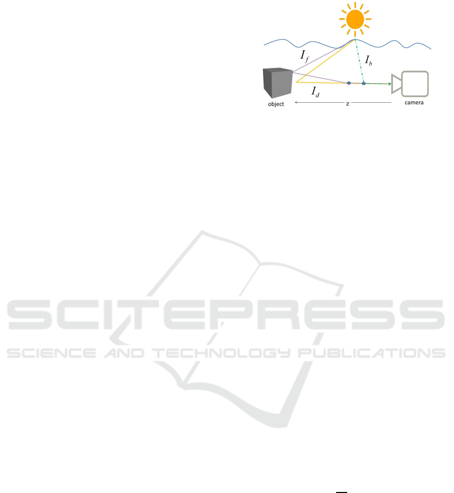
The ﬁnal light intensity I observedat the camera in

scattering media consists of three components, which

are the direct component I

, the backscattering com-

ponent I

, and the forward scattering component I

follows:

I = I

+ I

(1)

These three components are depicted in Fig. 2.

It is known that the effects of forward scattering

are small compared to the direct component and

backscattering component (Schechner and Karpel,

2005). Thus, we assume that the effects of I

are neg-

ligible, and only consider the direct component I

and

the backscattering component I

in Eq. (1).

2.1 Direct Component

The direct component I

is the light traveling from the

light source that arrives at the object and is reﬂected

directly back into the camera. This component con-

tains direct information about the target object such

as color and shape. In underwater environments, this

component becomes attenuated.

The amount of light that is able to arrive at the

camera depends on the transmission τ of the medium.

According to the Beer-Lambert law, the light intensity

will decrease exponentially with respect to distance

traveled, as follows:

τ = e

−c.z

(2)

where z denotes the distance of the object from the

camera, and c is the attenuation coefﬁcient. The coef-

ﬁcient c is the sum of both the absorption coefﬁcient

and the scattering coefﬁcient.

Figure 2: Underwater image formation model.

We can now calculate the direct component of

light based on the transmission of the water. Since

the coefﬁcient c is wavelength dependent, the direct

component can then be calculated as follows:

(λ) = I

(λ).ρ(λ).e

−c(λ)z

(3)

where the term I

annotates the intensity of the light

source, and ρ is the reﬂectance of the object.

2.2 Backscattering Component

The backscattering component I

is the light travel-

ing from the light source that encounters a micropar-

ticle and is scattered directly into the camera without

arriving at the object. This does not contain any in-

formation about the object, and results into a veiling

effect. This component reduces image contrast and

obscures geometric features of the object. In natural

underwater environments particularly, the scattering

effects are higher in the longer wavelengths, resulting

in a bluish hue.

In our model we assume the scattering to follow a

single scattering model such as in (Narasimhan et al.,

2005). In the single scattering model, light rays are

scattered to all directions from the microparticle. This

property is represented by using a phase function P .

As in (Narasimhan et al., 2005), we use the ﬁrst-order

approximation of the phase function, as follows:

P (g, α) =

4π

(1+ g.cosα) (4)

where α is the angle between the incoming and re-

ﬂected light ray, and g ∈ (−1, 1) to show the shape of

the phase function.

Using the phase function P (g, α), I

can be de-

scribed as follows:

(λ) =

x=0

b(λ).I

(λ).P (g, α).e

−c(λ)x

dx (5)

After deﬁning the I

and I

components, we can

calculate the ﬁnal amount of light that is captured by

VISAPP 2016 - International Conference on Computer Vision Theory and Applications

674

the camera as the sum of both components as follows:

I(λ) = I

(λ) + I

(λ)

= I

(λ).ρ(λ).e

−c(λ).z

x=0

b(λ).I

(λ).P (g, α).e

−c(λ)x

dx (6)

3 3D INFORMATION IN

UNDERWATER IMAGES

Before further analysis, we attempt to simplify the

physical model in Eq. (6). In reality, the attenua-

tion is wavelength dependent, but since we are using

3-channel RGB images, we simplify the model to the

R, G, and B channels separately. We also solve the

integration in the I

component, arriving at Eq. (7).

s∈{R,G,B}

= I

.ρ

−c

.P (g, α)

.(1− e

−c

)

(7)

Next, we consider the term

.P (g,α)

in the

backscattering component. This term can also be de-

scribed as the waterlight A. The waterlight A is the

intensity at a point where the light does not carry in-

formation of objects and originates solely from the

scattering effects. Finally, we represent the light re-

ﬂected by the object as the original object color inten-

sity J

= I

.ρ

, and take the transmission τ

as Eq. (2)

to arrive at the simpliﬁed equation for the observed

light, as follows:

s∈{R,G,B}

= J

.τ

+ A

.(1− τ

) (8)

Previous publications have used the image forma-

tion model shown in Eq. (8) to try to recover the clear

scene J

. This problem is under-constrained if the in-

put is only a single underwater image I

, so additional

constraints are necessary to solve the equation.

3.1 Red Channel Prior

Without any other prior information, it is difﬁcult to

extract depth information from a single image. For

foggy images, He et al. (He et al., 2011) proposed a

statistical prior named the Dark Channel Prior (DCP)

based on the physical observation of the image inten-

sities in clear images. The DCP states that in clear

outdoor images, for local patches of non-sky regions,

at least 1 channel in {R, G, B} will have a very low

intensity, as follows:

DCP(x) = min

y∈Ω(x)



min

s∈{R,G,B}

(y)



≈ 0 (9)

where x denotes the pixel location in the image, and

Ω(x) denotes the local patch of pixels around x.

The DCP was intended for scattering media in

the form of fog and smoke, and is not designed to

handle underwater environments. Due to the wave-

length dependent nature of attenuation in underwater

images, the J

channel is often very low in the en-

tire image, making the DCP invalid. In order to han-

dle this, more recent works have proposed modiﬁed

priors more suitable for underwater images, such as

the Underwater Dark Channel Prior (UDCP) (Drews

et al., 2013) and Red Channel Prior (RCP) (Galdran

et al., 2015). In our approach we use the Red Channel

Prior.

In order to handle the low R channel intensities,

the RCP (Galdran et al., 2015) replaces J

with its

reciprocalchannel 1−J

. The RCP states that in clear

non-degraded underwater images, for local patches of

non-water regions, at least 1 channel in {1− R, G, B}

will have a very low intensity, as follows:

RCP(x) = min( min

y∈Ω(x)

(1− J

(y)), min

y∈Ω(x)

(y)),

min

y∈Ω(x)

(y))) ≈ 0

(10)

3.2 Waterlight Estimation

Intuitively, waterlight A can be found at the pixel at

maximum distance from the camera (z → max), and

its color depends only on the scattering effects. As

mentioned in section 3.1, the red channel prior im-

plies that RCP(x) ≈ 0 at minimum distances z → 0

in non-degraded underwater images. Inversely, the

maximum distance and the waterlight can therefore be

found where RCP becomes maximum (Galdran et al.,

2015).

Despite this intuition, in reality the waterlight is

not always correctly found using the above assump-

tion. It is more difﬁcult while dealing with blue ob-

jects that are very similar to the waterlight. To handle

the erroneous estimated waterlight, we follow the so-

lution in (Galdran et al., 2015) by adding a user input

to select a general area of water, then the RCP is used

within that region to ﬁnd the correct waterlight pixel.

3.3 Transmission Estimation

Based on the red channel prior in section 3.1, we can

now estimate the transmission τ of an underwater im-

age (Galdran et al., 2015). Taking the image intensi-

ties I

s∈{1−R,G,B}

from Eq. (8), we divide them with

the waterlight A as follows:

Time-to-Contact from Underwater Images

675



1− I

1− A





1− J

1− A

+ (1− τ

), τ

+ (1− τ

)



(11)

Next we take the local minimum for every channel

in Eq. (11), and take the overall minimum on both

sides of the equation, as follows:

min



min

Ω

(

1− I

1− A

), min

Ω

(

), min

Ω

(

)



τ. min



min

Ω

(

1− J

1− A

), min

Ω

(

), min

Ω

(

)



+1− τ

(12)

where τ in Eq. (12) represents the transmission of the

minimum channel.

Since we have assumed the red channel prior to be

valid in underwater images (RCP ≈ 0), it cancels out

the ﬁrst term on the right hand side of Eq. (12), and

hence we have:

τ = 1− min



min

Ω

(

1− I

1− A

), min

Ω

(

), min

Ω

(

)



(13)

By using Eq.(13) we can estimate the transmission

τ of the minimum channel from the image intensity I

and the waterlight A.

4 TIME-TO-CONTACT FROM

UNDERWATER IMAGES

In the case of an object moving at a constant speed

towards the observer, or vice versa (Horn et al., 2007;

Cipolla and Blake, 1992), time-to-contact can be es-

timated by the ratio between the distance z and the

change in distance ∆z at time t as follows:

TTC =

∆z

(14)

From Eq. (14) it is apparent that we need two con-

secutive observationsat time t andt +1 for computing

time-to-contact. In clear environments, it is possible

to use the geometric properties of the observed object

such as height, width or area. Since these geometric

properties change in relation to distance z, they can

be used for computing time-to-contact. However, in

the case of underwater environments, these geomet-

ric properties are more difﬁcult to extract due to the

image degradation. Thus we propose the following

time-to-contact estimation method using image inten-

sity.

Suppose the target object has a surface facing the

camera, we can calculate the time-to-contact of the

object surface as follows. In section 3.3, the red chan-

nel prior is used to estimate the transmission in the

image. Since the distance information is encoded in

the transmission information as shown in Eq. (2), we

can deﬁne time-to-contact directly from the 2 consec-

utive observations of transmission.

Based on τ = e

−c.z

, the distance z can be repre-

sented by using the transmission τ as follows:

z =

logτ

−c

(15)

If the camera then moves closer by a distance of

∆z, the distance from the object becomes z − ∆z, and

thus we have:

z− ∆z =

logτ

′

−c

(16)

where τ

′

denotes the transmission at the second obser-

vation. ∆z then can be described by using the trans-

mission as:

∆z =

logτ − logτ

′

−c

(17)

By substituting Eq. (15) and Eq. (17) into Eq.

(14), the time-to-contact can be computed from the

change in transmission estimated from the change in

image intensity caused by the camera motion. The

TTC from transmission can then be written as fol-

lows:

TTC =

logτ

logτ − logτ

′

(18)

5 EXPERIMENTAL RESULTS

In order to evaluate the performance of the proposed

TTC estimation method proposed in section 4, we

conducted a series of experiments using both syn-

thetic and real underwater images.

Note that the proposed estimation method can

compute the time-to-contact from just a single point

on the object surface, but in order to account for the

noise and error we consider an area of points on the

object’s surface. Even so, there is no need for exact

point and line correspondencesbetween observations,

as we only need to track the object area. In our work

we assume that the region of interest (ROI) is prede-

ﬁned.

5.1 Synthetic Images

In the ﬁrst step of our experiments, a set of synthetic

images was generated simulating an object in an un-

derwater environment at different distances from the

VISAPP 2016 - International Conference on Computer Vision Theory and Applications

676

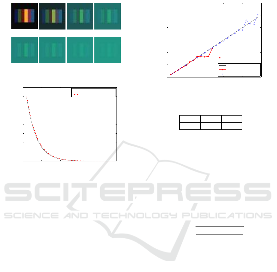
(a) Object

(b) 2m (c) 6m (d) 10m

(e) 14m (f) 16m

(g) 20m

(h) 24m

Figure 3: Synthetic underwater images.

0 5 10 15 20 25

0.1

0.2

0.3

0.4

0.5

0.6

0.7

0.8

Distance (m)

Transmission

Real Transmission

Estimated Transmission

Figure 4: Transmission estimated from synthetic underwa-

ter images.

camera. Considering a ﬂat object facing the camera

as shown in Fig. 3(a), we simulated the underwater

scattering effects based on the physical model in Eq.

(6) at distances between 0 to 24 meters (Fig. 3(b)-(h)).

These synthetic images show simulated scattering ef-

fects according to the distance and wavelength.

Before estimating time-to-contact, we ﬁrst ana-

lyze the estimated transmission in the synthetic un-

derwater images according to Eq. (13). Since the

estimation is pixel-wise, we take the median value

of transmission estimates from the region of interest.

The transmission estimation results compared to the

real transmission can be seen in Fig. 4.

With the transmission accurately estimated, we

then calculated the time-to-contact from the synthetic

underwater images based on the TTC from transmis-

sion method proposed in section 4. Given that the ob-

ject is moving towards the camera at a constant speed

of 1 m/s from the distance of 24 to 1 meters, we cal-

culated the TTC from both 8-bit and 16-bit images, as

shown in Fig. 5.

The results in Fig. 5 show that the proposed

method is able to estimate time-to-contact well. How-

ever, since the estimation fails at smaller distances

when we use 8-bit images due to quantization error,

it is desirable to use 16-bit representations to ensure

robustness.

In the next experiment we once again evaluate the

0 5 10 15 20 25

Real TTC

Estimated TTC

Real TTC

Est TTC 8−bit images

Est TTC16−bit images

Figure 5: TTC estimated from transmission using 8-bit and

16-bit synthetic underwater images.

Table 1: Estimation error in synthetic images.

1 m/s 2 m/s 4 m/s

0.63 0.16 0.06

time-to-contact estimation of the proposed TTC from

transmission. Using only 16-bit images, we estimate

the time-to-contact for the object moving at various

speeds. The results are shown in Fig. 6.

The results show that even with the 16-bit im-

ages, the time-to-contact estimation starts to fail at

distances above 23 meters, especially in Fig. 6(a).

This is due to the scattering effects that eliminate al-

most all of the object details in images.

Lastly, we calculate the standard error of the pro-

posed method. The standard error of estimates can be

calculated as:

E =

∑

(TTC

− TTC

)

(19)

where TTC

is the estimated TTC, TTC

is the real

TTC, and N is the number of observations. The error

of TTC from transmission using simulated images is

shown in Table 1.

It is apparent that the stability of the time-to-

contact estimation improves at higher speeds, due to

the larger distances between observations. This larger

distance causes a larger observable change in inten-

sity that improves the time-to-contact estimation.

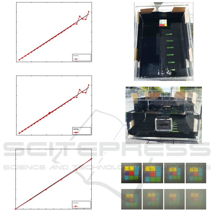
5.2 Real Images

We further evaluate the TTC from transmission

method proposed in section 4 using real images taken

in an experimental underwater environment. The im-

ages were captured using an action camera, which is

designed for capturing high-action shots. The action

camera is shockproof and equipped with a waterproof

case, enabling us to use it to capture stable underwater

images.

Time-to-Contact from Underwater Images

677

0 5 10 15 20 25

Real TTC

Estimated TTC

Real TTC

Est TTC

(a) Speed 1 m/s

0 5 10 15 20 25

Real TTC

Estimated TTC

Real TTC

Est TTC

(b) Speed 2 m/s

1 1.5 2 2.5 3 3.5 4 4.5 5 5.5 6

Real TTC

Estimated TTC

Real TTC

Est TTC

Figure 6: TTC estimated from synthetic underwater images

at various speeds.

In order to capture the experimental images, a 30

x 20 x 40 cm aquarium is placed in an sunny out-

door area. There is no additional light source aside

from the natural ambient sunlight. The bottom and

sides of the aquarium are covered with a black rubber

non-reﬂecting material, in order to ensure the incom-

ing light is coming from above only. The aquarium is

then ﬁlled with 10 liters of water and both the camera

and the object are submerged in the water, as shown

in Fig. 7.

To obtain more visible scattering effects, we

(a) Aerial View

(b) Frontal View

Figure 7: Experimental setup.

(a) 6cm (b) 9cm (c) 12cm (d) 15cm

(e) 18cm (f) 21cm

(g) 24cm

(h) 27cm

Figure 8: Captured images of object in 0.02% milk solution.

added turbidity to the water. We captured images us-

ing 2 different water solutions, which was a 0.02%

milk solution with 2 ml of milk dissolved into the wa-

ter, as well as the same milk solution with added blue

food coloring. We then captured images of the object

at distances ranging from 4 cm to 30 cm at an interval

of 1 cm. The resulting images are shown in Fig. 8 and

Fig. 9.

As previously done with the synthetic images, we

ﬁrst estimated the transmission in the real underwa-

ter images based on Eq.(13). Once again we take the

median value of the transmission estimates in the re-

gion of interest. The results are shown in Fig. 10.

VISAPP 2016 - International Conference on Computer Vision Theory and Applications

678

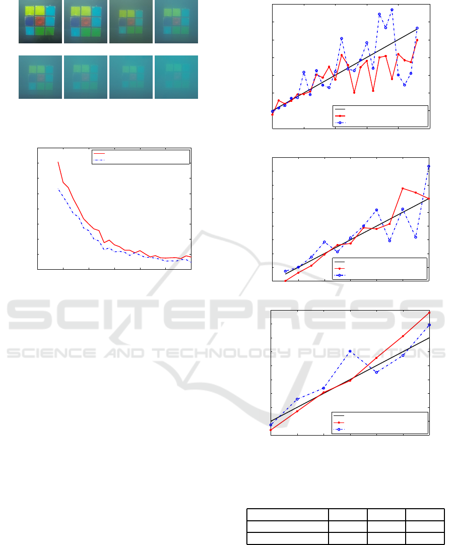
(a) 6cm (b) 9cm (c) 12cm (d) 15cm

(e) 18cm (f) 21cm

(g) 24cm

(h) 27cm

Figure 9: Captured images of object in 0.02% milk solution

plus blue food coloring.

0 5 10 15 20 25 30

0.1

0.2

0.3

0.4

0.5

0.6

0.7

0.8

Distance (cm)

Transmission

Est Transmission 0.02% milk

Est Transmission 0.02% milk+blue

Figure 10: Transmission estimated from real underwater

images.

Without information about the absorption and scatter-

ing coefﬁcients, we cannot compare the results with

the ground truth. However, it can be observed that the

transmission decreases with a slope consistent with an

exponential decay function.

Next, we evaluate the performance of the pro-

posed TTC from transmission method using real im-

ages. The action camera used in this experiment is

only able to capture 8-bit images, but since we are

dealing with small distances, the images are sufﬁcient

for TTC estimation. Using the captured images at dif-

ferent intervals, we simulate the object moving at var-

ious speeds. The TTC estimation results are shown in

Fig. 11.

We can see from Fig. 11 that due to the natural

noise in the real images, the estimation shows a level

of error. However, from the results we can still distin-

guish a slope that follows the correct time-to-contact.

Aside from the natural environmental noise, the er-

ror in estimation could also be caused by human error

during the process of image capture.

Finally, we calculate the standard error of esti-

mates using Eq.(19). The error of TTC from trans-

mission using simulated images is shown in Table 2.

In the case of real images, the time-to-contact estima-

tion also improves at higher speeds.

5 10 15 20 25 30

Real TTC

Estimated TTC

Real TTC

Est TTC 0.02% milk

Est TTC 0.02% milk + blue color

(a) Speed 1 cm/s

2 4 6 8 10 12 14

Real TTC

Estimated TTC

Real TTC

Est TTC 0.02% milk

Est TTC 0.02% milk + blue color

(b) Speed 2 cm/s

1 2 3 4 5 6 7

Real TTC

Estimated TTC

Real TTC

Est TTC 0.02% milk

Est TTC 0.02% milk + blue color

Figure 11: TTC estimated from real underwater images at

various speeds.

Table 2: Estimation error in real images.

Speed 1 cm/s 2 cm/s 4 cm/s

milk solution 4.48 1.23 0.87

milk + blue color 5.88 2.31 0.91

6 CONCLUSION AND FUTURE

WORK

In this paper, we proposed a novel method for estimat-

ing time-to-contact from underwater images, namely

Time-to-Contact from Underwater Images

679

TTC from transmission. Our method does not require

a dedicated light source nor camera calibration. The

proposed method uses the image intensity and the em-

bedded scattering effects to extract 3D distance infor-

mation from the image.

We have tested these methods using both syn-

thetic and real underwater images. The synthetic im-

ages were generated based on an underwater light

propagation model, and the real underwater images

were taken in an experimental underwater environ-

ment. The proposed method is able to accurately esti-

mate TTC in synthetic underwater images and shows

promising results for real underwater images. The dif-

ference that occurs with the real images is due to the

real natural noise and possibly due to human error in

the image capture process. Even so, the TTC estima-

tion shows a slope that follows the correct TTC val-

ues.

It is mentioned in this paper that the waterlight es-

timation outlined in section 3.2 requires an additional

user input to ensure correct waterlight is used. The red

channel prior assumption used in the waterlight esti-

mation is sometimes hindered by bright areas or ob-

jects with a reﬂectance similar to the waterlight. This

albedo-airlight ambiguity is an ongoing issue for vi-

sion in scattering media.

For the next step in our work, we will address this

albedo-airlight ambiguity problem in underwater vi-

sion. We aim to arrive at a solution for better wa-

terlight estimation results, which in turn will lead to

an improvedtransmission and 3D distance estimation.

Furthermore, we will examine the possibility of more

novel and improved methods for extracting 3D infor-

mation from underwater images, which can then be

applied to TTC estimation, 3D shape reconstruction,

as well as to other underwater vision applications.

REFERENCES

Ahn, Y.-H., Bricaud, A., and Morel, A. (1992). Light

backscattering efﬁciency and related properties of

some phytoplankters. Deep Sea Research Part A.

Oceanographic Research Papers, 39(11):1835–1855.

Cipolla, R. and Blake, A. (1992). Surface orientation and

time to contact from image divergence and deforma-

tion. In Proc. European Conference on Computer Vi-

sion (ECCV), pages 465–474.

Drews, P., do Nascimento, E., Moraes, F., Botelho, S., and

Campos, M. (2013). Transmission estimation in un-

derwater single images. In Proc. IEEE International

Conference on Computer Vision Workshops (ICCVW),

pages 825–830. IEEE.

Galdran, A., Pardo, D., Pic´on, A., and Alvarez-Gila, A.

(2015). Automatic red-channel underwater image

restoration. Journal of Visual Communication and Im-

age Representation, 26:132–145.

He, K., Sun, J., and Tang, X. (2011). Single image haze

removal using dark channel prior. In Proc. IEEE Con-

ference on Computer Vision and Pattern Recognition

(CVPR), pages 1956–1963. IEEE.

Horn, B., Fang, Y., and Masaki, I. (2007). Time to con-

tact relative to a planar surface. In Proc. Intelligent

Vehicles Symposium, pages 68–74.

Jeong, W., Rahadianti, L., Sakaue, F., and Sato, J. (2015).

Time-to-contact in scattering media. In Proc. IEEE

Conference on Computer Vision Theory and Applica-

tions, pages 658–663.

Narasimhan, S., Nayar, S., Sun, B., and Koppal, S. (2005).

Structured light in scattering media. In Proc. Interna-

tional Conference on Computer Vision (ICCV), pages

420–427.

Narasimhan, S. G. and Nayar, S. (2003a). Interactive

deweathering of an image using physical models.

In Proc. IEEE Workshop on Color and Photometric

Methods in Computer Vision.

Narasimhan, S. G. and Nayar, S. K. (2003b). Contrast

restoration of weather degraded images. IEEE PAMI,

25(6):713 – 724.

Schechner, Y. Y. and Karpel, N. (2005). Recovery of under-

water visibility and structure by polarization analysis.

IEEE Journal of Oceanic Engineering, 30(3):570–

587.

Smith, R. C. and Baker, K. S. (1981). Optical properties

of the clearest natural waters (200–800 nm). Applied

Optics, 20(2):177–184.

Watanabe, Y., Sakaue, F., and Sato, J. (2015). Time-to-

contact from image intensity. In Proc. IEEE Con-

ference on Computer Vision and Pattern Recognition

(CVPR), pages 4176–4183.

VISAPP 2016 - International Conference on Computer Vision Theory and Applications

680