Constrained Portfolio Optimisation: The State-of-the-Art Markowitz

Models

Yan Jin, Rong Qu and Jason Atkin

ASAP Group, School of Computer Science, The University of Nottingham, Nottingham, U.K.

Keywords:

Constrained Portfolio Optimization, Mean-variance, Cardinality, Pre-assignment, Round-lot, Class.

Abstract:

This paper studies the state-of-art constrained portfolio optimization models, using exact solver to identify the

optimal solutions or lower bound for the benchmark instances at the OR-library with extended constraints. The

effects of pre-assignment, round-lot, and class constraints based on the quantity and cardinality constrained

Markowitz model are ﬁrstly investigated to gain insights of increased problem difﬁculty, followed by the

analysis of various constraint settings including those mostly studied in the literature. The study aims to

provide useful guidance for future investigations in computational algorithms.

1 INTRODUCTION

Portfolio optimization (PO) is an extensively studied

area in ﬁnance. The seminal work by (Markowitz,

1952) had a profound impact on the development of

PO in the last 60 years. The Mean-Variance (MV)

model introduced by Markowitz focusses on ﬁnding

the best trade-off between the return and risk of port-

folios, i.e. mean of return and covariance of return,

to minimise the risk given an expected return level or

vice versa.

Although the signiﬁcance of the MV model is

unanimously recognized, the basic model has been

widely challenged for some underlying assumptions.

It neglects many realistic restrictions faced by in-

vestors like tax and transaction cost; personal or

strategic investment decisions, etc. It assumes as-

sets are traded at any fractions. It implicitly encour-

ages holdings of as many assets as possible to diver-

sify the overall risk. In reality, an investment man-

ager may face the restrictions on the minimum and/or

maximum capital allocated to an asset or industry. In-

vestors also prefer a limited number of assets (Jansen

and van Dijk, 2002).

The complexity of the PO problem to a large ex-

tent depends on the constraints (Maringer, 2008). The

basic MV model is a standard quadratic programming

problem. There has been numerous tools to solve it

optimally. However real-world ﬁnancial constraints

signiﬁcantly increase the level of complexity. For in-

stance, cardinality constraint requires only a limited

number of assets to be included in the portfolio, which

turns the problem into non-convex. It is no longer

always suitable to use exact methods to ﬁnd optimal

solutions thus the majority of work in the current lit-

erature has focused on heuristics for the constrained

PO problem.

Nevertheless, due to the fast development some

constraints now can be handled by commercial

solvers such as CPLEX with limited computational

cost for many difﬁcult optimisation problems. The

purpose of our study is to provide an insight into the

current state of the MV models with subsets of prac-

tical constraints using CPLEX, and provide useful

guidance of potential areas of future research on com-

putational algorithms for constrained PO problems.

This paper is organised as follows. Firstly, we

overview the basic MV model and the extended con-

straints in Section 2. Then a comprehensive overview

of related literature for various settings of practical

constraints is presented in Section 3. It summarises

the representative works in terms of different con-

straints applied. Section 4 presents the experimen-

tal study by reviewing the models in the literature

and provides the optimal solutions or lower bound for

those mostly studied models. Finally, in Section 5, we

identify some possible future research on algorithms

for the constrained MV models in portfolio optimisa-

tion.

388

Jin, Y., Qu, R. and Atkin, J.

Constrained Portfolio Optimisation: The State-of-the-Art Markowitz Models.

DOI: 10.5220/0005758303880395

In Proceedings of 5th the International Conference on Operations Research and Enterprise Systems (ICORES 2016), pages 388-395

ISBN: 978-989-758-171-7

2 PROBLEM FORMULATION

2.1 Mean-Variance Model

The MV model considers a single period of invest-

ment. The process of PO allocates among N different

assets the proportions (x

, i = 1, ...N) of the capital to

form a portfolio. Each asset i has a return rate r

and

is associated with a covariance σ

i j

of the return with

each other asset j. The total return r

of a portfolio is

given by the weighted combination of the constituent

assets’ returns

∑

i=1

, and its risk v

is deﬁned

∑

i=1

∑

j=1

i j

. The aim is to minimize the

portfolio risk v

for a given level of expected return

exp

or vice versa, mathematical formulation of the

model as follows:

Minimise

∑

i=1

∑

j=1

i j

(1)

Subject to

∑

i=1

= R

exp

(2)

∑

i=1

= 1 (3)

0 6 x

6 1, i = 1, ..., N (4)

Constraint (2) deﬁnes the expected return. The

budget constraint (3) requires the whole capital

should be invested. Investment to each asset is non-

negative, deﬁned in constraint (4). A set of optimal

portfolios of the lowest risk for various values of R

exp

can be obtained by solving the above model repeat-

edly, which forms the efﬁcient frontier (EF). For each

point on EF, there should be no portfolio with a higher

expected return at the same risk level, and no portfolio

with a lower risk at the same level of return.

2.2 Additional Practical Constraints

Several extensions have been proposed to enrich the

MV model with real world constraints in the liter-

ature. In this paper, we investigate the following

mostly studied additional practical constraints based

on the basic MV model.

Cardinality Constraint. The cardinality constraint

restricts the number of K assets in a portfolio. A bi-

nary variable z

is introduced to denote whether an

asset is selected or not. This constraint is relaxed to

i.e.

∑

i=1

≤ K in some work in the literature.

∑

i=1

= K (5)

∈ {0, 1}, i = 1, ..., N (6)

Quantity Constraint. The quantity constraint

speciﬁes the lower (ε) and upper (δ) bounds allowed

for the allocated proportions to each asset in a

portfolio.

εz

6 x

6 δz

, i = 1, ..., N (7)

Pre-assignment Constraint. Pre-assignment con-

straint pre-selects investor’s preferred assets in the

portfolio. It was ﬁrstly discussed in (Chang et al.,

2000) and ﬁrstly applied in (Di Gaspero et al., 2011).

A binary variable s

is introduced to denote if asset i

belongs to the pre-assigned set P, 0 otherwise.

= 1, i ∈ P (8)

> s

, i = 1, ..., N (9)

Round Lot Constraint. Round lot constraint de-

ﬁnes that the investment of any asset in the portfolio

should be an exact multiple units of a minimum lot.

An integer variable y

and minimum lot l

for each

asset are introduced. The round lot constraint might

cause the budget constraint (3) not strictly satisﬁed,

as the capital cannot always be divided as an exact

multiple of trading lot for all the assets.

= y

∗ l

, i = 1, ..., N (10)

Class Constraint. Introduced by (Chang et al.,

2000), class constraint is used to limit the total pro-

portion invested in those assets with common charac-

teristics, leading to a more diversiﬁed and safe port-

folio. Classes of assets are considered to be mutually

exclusive, i.e. C

∩C

= ∅ for all assets i 6= j. In this

study we require at least one asset from each of the

M classes to be selected, thus K ≥ M. Here the upper

bound is set as 1, and the lower bound of each class

is L

> 0 for every class C

, m = 1,..., M. Then the

lower bound is formulated as follows:

∑

i∈C

6 1, m = 1, ...M (11)

3 STUDIES OF VARIOUS

EXTENDED MV MODELS

The basic MV model is a quadratic programming

problem and can be solved efﬁciently by some spe-

Constrained Portfolio Optimisation: The State-of-the-Art Markowitz Models

389

cialized exact methods such as simplex method and

branch and bound methods. These techniques can

also handle arbitrary linear constraints, like quantity

constraint, see (Borchers and Mitchell, 1997). Never-

theless the problem becomes increasingly much more

complex when the number of assets increases and

with additional constraints. For instance, with the

cardinality constraint, the problem turns into a mixed

integer nonlinear programming and NP-hard (Bien-

stock, 1995). (Bienstock, 1995) presented a branch

and cut algorithm for the cardinality constrained PO

problem of up to 3897 assets with various cardinality

values. At the time of publication results shown that

this type of problem with larger size may be impossi-

ble to solve to a proved optimality within a reasonable

time. Some works require strictly K assets to be in-

cluded in a portfolio ((Chang et al., 2000; Fernandez

and Gomez, 2007; Xu et al., 2010; Woodside-Oriakhi

et al., 2011; Jin et al., 2014)) while some others use

relaxed version ((Schaerf, 2002; Ruiz-Torrubiano and

Suarez, 2010)).

There are not many experimental studies on the

pre-assignment constraint so far, except some infor-

mal discussion (Di Tollo and Roli, 2008).(Di Gaspero

et al., 2011) examined the impact of the pre-

assignment constraint and reported that pre-assigning

one asset tended to worsen the performance except

when the asset is in the optimal solution for all the

expected return levels.

Recently, some scholars included the round-lot

constraint into PO problems, which makes it more

difﬁcult to ﬁnd a feasible solution. Some of these

were measured in units of money ((Speranza, 1996;

Mansini and Speranza, 1999; Kellerer et al., 2000;

Lin and Liu, 2008; Bonami and Lejeune, 2009; Gol-

makani and Fazel, 2011)), while others imposed that

the continuous weight variables should be an integer

multiple of a given fraction ((Jobst et al., 2001; Stre-

ichert et al., 2004; Skolpadungket et al., 2007)). Some

of them included transaction cost at the same time.

(Mansini and Speranza, 1999) showed that a PO prob-

lem with minimum lot and without any ﬁxed transac-

tion cost is NP-complete.

Class constraint was ﬁrst introduced by (Chang

et al., 2000), also mentioned in (Ruiz-Torrubiano

and Suarez, 2010), and applied in ((Anagnostopoulos

and Mamanis, 2010; Anagnostopoulos and Mamanis,

2011a; Anagnostopoulos and Mamanis, 2011b)). An-

other form of this constraint is splitting the universe

of assets into subsets with similar features. Optimi-

sation is performed on the best representative of each

class (Vijayalakshmi Pai and Michel, 2009).

Most of the research in the literature adopt two

constraints in the problem formulation. In particu-

lar, cardinality and quantity constraints were stud-

ied 44.93% and 30.43%, respectively, in the portfo-

lio management models (Metaxiotis and Liagkouras,

2012).

4 ANALYSIS ON DIFFERENT

CONSTRAINTS IN THE MV

MODEL

As most of the applications in the literature dealt

with quantity and cardinality constrained PO prob-

lems, in this section we ﬁrst discuss the effect of

pre-assignment, round-lot and class constraint based

on the quantity and cardinality constrained MV

model in terms of solution quality and computational

cost. Then we present experimental framework us-

ing CPLEX 12.6 to identify solutions for the most

commonly applied constrained MV models in the lit-

erature, some models with different settings in con-

straints.

Five widely tested benchmark datasets in the OR-

library (Beasley, 1990) (http://people.brunel.ac.uk/

∼mastjjb/jeb/info.html) are chosen in our experi-

ments. They were extracted from the well-known

indices, the Hong Kong HangSeng, the German

DAX100, the UK FTSE100, the US S&P100 and

the Japan Nikkei, with dimension N = 31, 85, 89, 98

and 225 (N31-N225), respectively. The portfo-

lios obtained under different constraints and settings

form constrained efﬁcient frontiers (CEF). The un-

constrained efﬁcient frontier (UEF), for the uncon-

strained PO problem from the OR-library, is used as

the upper bounds for CEF. For each dataset, 50 points

across the UEF are chosen. For each point on the

CEF, the solver is run to minimise risk (QP) given

a respected return. The stopping time limit is set to

3600 seconds.

Several performance measures are adopted, for

which smaller values denote better solutions. The

Average Percentage Error (APE) (Di Gaspero et al.,

2011) measures the relative distance between the ob-

tained CEF from the UEF with the same expected re-

turn, calculated using Formula (11), where x

∗

and x

denote the portfolios on the CEF and UEF, respec-

tively, f

denotes the value of the obtained risk, and p

is the number of portfolios on the frontier.

APE =

∗

∑

i=1

∗

) − f

(x)

(11)

Generational distance (GD) (Cura, 2009) refers to

the average minimum distance of each portfolio on

the CEF from the UEF, calculated using Formula (12)

ICORES 2016 - 5th International Conference on Operations Research and Enterprise Systems

390

where d

∗

is the Euclidean distance. f

and f

are the

risk (Eq.(1)) and return (Eq.(2)) of the portfolio. It

measures how close the obtained CEF is to the UEF.

GD =

∗

∑

∗

∈X

CEF

min{d

∗

|x ∈ X

UEF

} (12)

∗

( f

∗

) − f

(x))

+ ( f

∗

) − f

(x))

(13)

Inverted generational distance(IGD) is a variant of

GD. It uses UEF as a reference to calculate the av-

erage minimum distance of its each portfolio to the

CEF, calculated using Formula (14). This measure

mainly shows the overall quality of the obtained so-

lution set (i.e. its diversity and convergence to the

UEF).

IGD =

∗

∑

∗

∈X

UEF

min{d

∗

|x ∈ X

CEF

} (14)

Algorithm Effort (AE) (Chen et al., 2012), AE =

Time

, measures the ratio of the total run time to the

number of feasible portfolios obtained on the CEF.

MAX and MIN denote the maximum or minimum

time spent for one portfolio. Optimal Rate is used

to denote the rate of optimal solutions obtained out of

all the points on the CEF.

The experiments are coded in C++ in Microsoft

Visual Studio 2012, and run on a PC with Windows

7 Operating System (64-bit), 6GB of RAM, and an

Intel Core i7 CPU (960@3.2GHz).

4.1 Pre-assignment, Round-lot and

Class Constraints

We ﬁrst test all the extended constraints on the MV

model. The lower and upper bounds of the weights

are set as ε = 0.01, δ = 1, and cardinality K = 10.

These are widely used in the literature. Preliminary

computational results indicate that the pre-assigned

asset(s) is not a main performance discriminator of

the basic MV model, thus is randomly set as P =

{30}. The class constraints is set to: randomly de-

ﬁne two classes with size of 20% proportionately to

problem dimension (N). These constraints are set

as those in (Lwin et al., 2014). Initial experiment

results showed that cardinality constraint contributes

the most to the problem difﬁculty.

We then assess the effect on the computational

cost from pre-assignment (C3), round-lot (C4) and

class (C5) constraints based on the MV model with

cardinality (C1) and quantity (C2) constraints, i.e.

ε = 0.01, K = 10.

4.1.1 Pre-assignment Constraint(C3)

To evaluate the impact of pre-assignment constraint

on the computational cost, for each benchmark in-

stance, we ﬁx in turn one of the assets as pre-assigned

(imposing C1 and C2 with the settings as mentioned

above). For each instance we then obtain a group of N

CEFs, one for each pre-assigned asset. Intuitively, the

choice of the pre-assigned assets determines the so-

lution quality measured in APE. For example, if the

pre-assigned asset does not belong to any optimal so-

lution for most of the values of the required return

exp

on UEF, the pre-assignment constraint generally

deteriorates the solution quality. Moreover, the mag-

nitude of this worsening may depend on the features

of the asset, e.g. return rate, standard deviation(sd),

and the ratio of return/sd, etc.

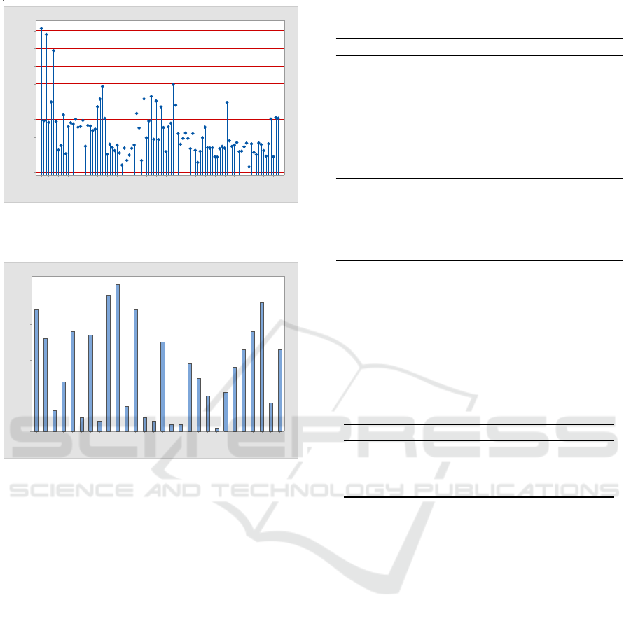
As an example, in Figure 1, for instance N98, the

average time spent for computing the CEF for each

pre-assigned asset is plotted. It can be seen that the

time used varies with obvious difference among dif-

ferent assets, ranging from around 20s to 400s. Figure

2 reports the frequency of each asset appearing in the

optimal portfolios on the UEF. For instance, asset 1

which leads to the maximum time used (400s) never

appears in the optimal solution in the unconstrained

problem. Moreover, the rankings of its return rate,

sd, and the ratio of return/sd are quite low, ranked as

61, 64, and 71, respectively. The assets ranked top

in return rate, sd and ratio (namely assets 82, 62, and

89) appear to lead to around only 50s, which is at the

lower level of time used in Figure 1. Moreover, asset

89 appears 36 times out of 50 in the optimal portfo-

lios on the UEF shown in Figure 2. These imply that

there is some correlation between the feature of the

pre-assigned asset and the solution construction.

Intuitively, if we pre-assign more assets in ad-

vance, the problem becomes smaller with only (K −

pre assigned) number of assets. We conduct an an-

other experiment on two groups of pre-assigned assets

on instance N98, each with the top ﬁve and bottom

ﬁve shown in Figure 2. As expected in Table 1, the

computational time with more pre-assigned assets is

much lower than that with fewer assets. Pre-assigning

the assets which intend to appear in the optimal port-

folio on UEF can reduce the computational cost and

lead to better solution quality.

Table 1: Results of pre-assigned assets with different fea-

tures.

Pre-assigned APE MAX AE Optimal Rate

Top 5 0.100718 19.005 4.609 0.98

Bottom 5 0.234882 122.136 22.716 0.96

Constrained Portfolio Optimisation: The State-of-the-Art Markowitz Models

391

96928884807672686460565248444036322824201612841

400

350

300

250

200

150

100

Index of asset

Time(s)

Figure 1: Average time used for N98, with each pre-

assigned asset.

9693898682767366656462525145444342373634332322201914112

index of asset

Count No.

Figure 2: Frequency of each in the optimal solution on UEF

in N98, y-axix is the occurrence number.

4.1.2 Round-lot Constraint(C4)

We test on all the instances with three different lot

unit sizes and compare the results against the model

without round-lot constraint. As seen in Table 2, there

are no signiﬁcant differences in terms of the computa-

tional time and optimal rate. The chosen lot unit size

has a slight effect on the optimal rate.

4.1.3 Class Constraint(C5)

The class constraint is tested with different settings on

the class deﬁned and the lower bound. From the theo-

retical perspective, class constraint is linear thus does

not increase the problem difﬁculty. The number of

classes should also reduce the problem difﬁculty as

the original problem is partitioned into a set of sub-

problems with lower dimension. Table 3 shows the

results obtained on instance N98 with different class

settings based on the C1 and C2 constrained models.

The class classiﬁcation here is randomly assigned.

From Table 3, it can be seen that the higher lower

bound 0.1 could reduce the optimal rate compared

Table 2: Results on the C4 constrained problem based on

C1 and C2 constrained MV model.

Dataset Lot unit APE Max Time AE Optimal Rate

N31

NA 0.02107 0.983 0.138 0.92

0.005 0.02157 0.719 0.269 0.92

0.008 0.03321 9.612 2.675 0.88

0.01 0.02194 0.577 0.108 0.92

N85

NA 0.07539 61.463 11.500 0.94

0.005 0.07686 49.954 5.550 0.94

0.008 0.07686 49.954 5.550 0.94

0.01 0.07838 44.33 5.03887 0.94

N89

NA 0.02569 902.803 101.885 0.94

0.005 0.02625 1586.61 97.140 0.94

0.008 0.02936 400.068 39.773 0.92

0.01 0.02681 1177.83 91.809 0.94

N98

NA 0.06181 3600.59 1055.72 0.7

0.005 0.06265 3600.47 1042.23 0.72

0.008 0.06749 3600.64 979.171 0.76

0.01 0.06345 3600.4 1037.42 0.72

N225

NA 0.01034 16.333 7.229 0.98

0.005 0.01107 12.592 5.284 0.98

0.008 0.01129 23.865 8.139 0.96

0.01 0.01138 9.441 4.146 0.98

to 0.05. As expected, the setting with less classes

requires much more computational effort than those

with more classes. Intuitively expected, in terms of

computational cost, the class constraint does not gen-

erate much difﬁculty on the cardinality constrained

model, while it can affect the rate of optimality.

Table 3: Results with different class settings based on the

C1 and C2 constrained MV Model.

Class setting APE MAX AE Optimal Rate

NA 0.061814 3600.59 1055.72 0.7

size=6, LC=0.05 0.163718 519.235 101.793 0.84

size=6, LC=0.1 0.246108 999.286 156.248 0.68

size=2, LC=0.1 0.096405 3601.05 1123.34 0.62

size=2, LC=0.05 0.079334 3599.82 433.568 0.9

4.2 Performance of CPLEX for the

Complete Model

Table4 reports our results under different constraint

settings (Columns C1-C5) in terms of optimality, so-

lution quality (GD, IGD, APE), and computational

cost (MAX, MIN, AE) for the constrained models.

This feature is varied by the researchers. In the last

two models, for each instance, the asset which took

the longest time in Figure 1 is pre-assigned. Two

classes are deﬁned in the class constraint with the

lower bound set as 0.05. The results illustrate that,

the last two models spent much less computational

cost compared to the C1 and C2 constrained models.

In other words, combination of all these constraints

seems to have neutralizing effect.

4.3 Performance on Existing MV

Models in the Literature

In addition, to provide the optimal or lower bound

for various subsets of the constrained MV models

ICORES 2016 - 5th International Conference on Operations Research and Enterprise Systems

392

Table 4: Results of the complete MV Model with all ﬁve extended constraints.

Setting C1 C2 C3 C4 C5 Data GD IGD APE MAX MIN AE Optimal Rate

≥ R

exp

K = 10 ε = 0.01

N31 3.25e-05 9.64e-05 0.02107 0.98 0 0.13 0.92

N85 2.87e-05 7.4e-05 0.075388 61.5 0.04 11.49 0.94

N89 9.08e-05 4.45e-05 0.025686 902.8 0.06 101.85 0.94

N98 1.8e-05 5.46e-05 0.061814 3600.5 0.07 1055.72 0.7

N225 3.72e-06 2.48e-05 0.010336 16.3 2.57 7.22 0.98

= R

exp

K = 10 ε = 0.01

N31 3.24e-005 9.64e-005 0.020935 2.65 0.01 0.36 0.92

N85 2.87e-005 7.40e-005 0.075509 74.5 0.18 13.90 0.94

N89 8.99e-006 4.44e-005 0.025524 577.3 0.34 64.34 0.94

N98 1.80e-005 5.47e-005 0.061832 3600.5 0.06 893.54 0.78

N225 3.71e-006 2.48e-005 0.010293 20.3 2.75 10.55 0.98

≥ R

exp

K ≤ 10 ε = 0.01

N31 8.66e-008 4.94e-005 0.000124 5.94 0.03 0.48 1

N85 3.93e-006 4.74e-005 0.024219 84.1 0.19 11.68 1

N89 4.41e-006 3.24e-005 0.018769 652.2 0.17 109.47 1

N98 7.97e-006 4.83e-005 0.047498 3600.2 0.03 1128.91 0.7

N225 7.35e-007 2.35e-005 0.002157 27.4 0.21 7.37 1

= R

exp

K ≤ 10 ε = 0.01

N31 8.86e-08 4.94e-05 0.000128 7.48 0.01 0.51 1

N85 3.92e-06 4.74e-05 0.024198 89.9 0.07 12.28 1

N89 4.39e-06 3.24e-05 0.018719 609.4 0.07 107.88 1

N98 7.97e-06 4.83e-05 0.0475 3600.5 0.04 1103.17 0.7

N225 7.25e-07 2.35e-05 0.00217 14.1 0.14 6.24 1

≥ R

exp

K = 10 ε = 0.01

[2]

0.005

= 1..5

= 6..10

= 0.05

N31 4.61e-05 0.000106 0.032018 0.18 0.01 0.05 0.92

[83] N85 5.15e-05 0.000114 0.135537 3.9 0.04 0.92 0.9

[74] N89 1.81e-05 5.84e-05 0.049098 22.2 0.08 4.83 0.92

[1] N98 3.99e-05 8.46e-05 0.108055 248.3 0.05 41.12 0.94

[36] N225 2.16e-05 3.65e-05 0.053238 5.7 1.64 3.51 0.96

≥ R

exp

K = 10 ε = 0.01

[2]

0.008

= 1..5

= 6..10

= 0.05

N31 5.72e-05 0.000153 0.041071 3.08 0.06 0.44 0.88

[83] N85 4.72e-05 0.000153 0.124248 14.6 0.45 3.55 0.86

[74] N89 2.18e-05 7.13e-05 0.057599 34.2 0.26 7.63 0.9

[1] N98 4.36e-05 0.0001 0.115075 314.9 0.10 54.49 0.92

[36] N225 2.60e-05 4.50e-05 0.063057 6.1 1.01 3.58 0.94

Constrained Portfolio Optimisation: The State-of-the-Art Markowitz Models

393

Table 5: Results for various models in literature.

Models in the literature Data GD IGD APE AE Optimal Rate

(Maringer and Kellerer, 2003) N31 5.82E-08 4.94E-05 8.20E-05 0.01176 1

N85 3.91E-06 4.74E-05 0.024185 0.66952 1

N89 4.40E-06 3.24E-05 0.018769 1.95914 1

N98 7.96E-06 4.83E-05 0.047486 10.6813 1

N225 6.76E-07 2.35E-05 0.002015 1.2937 1

(Chang et al., 2000) N31 3.25E-05 9.64E-05 0.02107 0.137674 0.92

(Fernandez and Gomez, 2007) N85 2.87E-05 7.40E-05 0.075388 11.4999 0.94

(Xu et al., 2010) N89 9.08E-06 4.45E-05 0.025686 101.885 0.94

K = 10 N98 1.80E-05 5.46E-05 0.061814 1055.72 0.7

ε = 0.01 N225 3.72E-06 2.48E-05 0.010336 7.22906 0.98

(Ruiz-Torrubiano and Suarez, 2010) N31 8.86E-08 4.94E-05 0.000128 0.51264 1

(Schaerf, 2002) N85 3.92E-06 4.74E-05 0.024198 12.2765 1

K <= 10 N89 4.39E-06 3.24E-05 0.018719 107.883 1

ε = 0.01 N98 7.97E-06 4.83E-05 0.0475 1103.17 0.7

N225 7.25E-07 2.35E-05 0.00217 6.2358 1

(Lwin et al., 2014) N31 5.38E-05 0.00015 0.036569 1.90675 0.88

K = 10 N85 4.14E-05 0.000108 0.104911 16.5399 0.9

ε = 0.01 N89 2.22E-05 5.93E-05 0.054954 12.4044 0.92

N98 2.68E-05 6.68E-05 0.084467 107.943 0.96

N225 1.74E-05 3.86E-05 0.04161 7.39513 0.94

(Woodside-Oriakhi et al., 2011) N31 2.66E-05 0.000159 NA 0.0766 1

K = 10 N85 1.08E-05 0.000128 NA 9.91606 1

ε = 0.01 N89 6.81E-06 9.35E-05 NA 94.7458 1

exp

in range:[0.9R

exp

,1.1R

exp

] N98 1.46E-05 0.00014 NA 1105.7 0.72

N225 2.06E-06 5.27E-05 NA 6.54972 1

in the literature, the most commonly applied settings

in different constraints in relevant works are tested.

Due to the space limited, a sketch of the performance

of the representative models with different combi-

nations of constraints is shown in Table 5. More

detailed data and updated models are published in

http://www.cs.nott.ac.uk/∼pszrq/benchmarks.htm.

5 CONCLUSION AND FUTURE

WORK

This paper studies the constrained Markowitz MV

model for the portfolio optimisation problem, where

quantity, cardinality, pre-assignment, round-lot and

class constraints are considered. We ﬁrst discuss the

effect of the pre-assignment, round-lot and class con-

straints based on the cardinality and quantity con-

strained models in terms of computational cost. Then

we conduct experiments using CPLEX to obtain op-

timal or feasible solutions within a limited computa-

tional cost for various models with different constraint

settings. The results for the thoroughly studied con-

strained models are presented.

According to the results, the pre-assignment,

round-lot and class constraints do not make a big dif-

ference to the cost of solving the quantity and cardi-

nality constrained problem. As the mostly considered

constraint in the current literature, the cardinality con-

straint is proved to contribute to mainly the problem

difﬁculty. In addition, the more speciﬁc settings im-

posed on these constraints, the easier the problem is.

The complete constrained MV model with all the con-

straints can neutralize the effect of cardinality con-

straint, and the optimal solutions can be much easier

to obtain.

There are some exceptional points on instance

N98, which still requires a huge amount of compu-

tational effort for the cardinality constrained models.

Nevertheless, due to the fast development of commer-

cial solvers, most of the currently studied constrained

MV models can be efﬁciently solved to obtain most

of the optimal solutions within a limited time.

The above results motivate our future research to

more challenging PO problem. In the future, we plan

to further study the constrained PO problem based on

other risk measures such as VaR and CVaR which are

favoured by investors in reality. It is also interesting

to consider other constraints such as transaction cost

which occurs for problem with more than one invest-

ment period. We also aim to analyse the performance

on difﬁcult real instances of larger problem size.

REFERENCES

Anagnostopoulos, K. and Mamanis, G. (2010). A portfo-

lio optimization model with three objectives and dis-

crete variables. Computers & Operations Research,

37(7):1285 – 1297. Algorithmic and Computational

Methods in Retrial Queues.

Anagnostopoulos, K. and Mamanis, G. (2011a). The mean-

variance cardinality constrained portfolio optimiza-

tion problem: An experimental evaluation of ﬁve mul-

tiobjective evolutionary algorithms. Expert Systems

with Applications, 38(11):14208 – 14217.

Anagnostopoulos, K. P. and Mamanis, G. (2011b). Multiob-

jective evolutionary algorithms for complex portfolio

optimization problems. Computational Management

Science, 8(3):259–279.

Beasley, J. E. (1990). Or-library: Distributing test prob-

ICORES 2016 - 5th International Conference on Operations Research and Enterprise Systems

394

lems by electronic mail. Journal of the Operational

Research Society, 41:1069–1072.

Bienstock, D. (1995). Computational study of a family of

mixed-integer quadratic programming problems. In

Integer Programming and Combinatorial Optimiza-

tion, volume 920 of Lecture Notes in Computer Sci-

ence, pages 80–94. Springer Berlin Heidelberg.

Bonami, P. and Lejeune, M. A. (2009). An exact solu-

tion approach for portfolio optimization problems un-

der stochastic and integer constraints. Operations Re-

search, 57(3):650–670.

Borchers, B. and Mitchell, J. E. (1997). A computational

comparison of branch and bound and outer approxi-

mation algorithms for 01 mixed integer nonlinear pro-

grams. Computers & Operations Research, 24(8):699

– 701.

Chang, T.-J., Meade, N., Beasley, J., and Sharaiha, Y.

(2000). Heuristics for cardinality constrained portfo-

lio optimisation. Computers & Operations Research,

27(13):1271 – 1302.

Chen, A., Liang, Y.-C., and Liu, C.-C. (2012). An

artiﬁcial bee colony algorithm for the cardinality-

constrained portfolio optimization problems. In 2012

IEEE Congress on Evolutionary Computation (CEC),

pages 1–8.

Cura, T. (2009). Particle swarm optimization approach

to portfolio optimization. Nonlinear Analysis: Real

World Applications, 10(4):2396 – 2406.

Di Gaspero, L., Di Tollo, G., Roli, A., and Schaerf,

A. (2011). Hybrid metaheuristics for constrained

portfolio selection problems. Quantitative Finance,

11(10):1473–1487.

Di Tollo, G. and Roli, A. (2008). Metaheuristics for the

portfolio selection problem. International Journal of

Operationas Research, 5(1):13–35.

Fernandez, A. and Gomez, S. (2007). Portfolio selection

using neural networks. Computers & Operations Re-

search, 34(4):1177 – 1191.

Golmakani, H. R. and Fazel, M. (2011). Constrained port-

folio selection using particle swarm optimization. Ex-

pert Systems with Applications, 38(7):8327 – 8335.

Jansen, R. and van Dijk, R. (2002). Optimal benchmark

tracking with small portfolios. The Journal of Portfo-

lio Management, 28(2):33–39.

Jin, Y., Qu, R., and Atkin, J. (2014). A population-based

incremental learning method for constrained portfolio

optimisation. In Symbolic and Numeric Algorithms

for Scientiﬁc Computing (SYNASC), 2014 16th Inter-

national Symposium on, pages 212–219.

Jobst, N., Horniman, M., Lucas, C., and Mitra, G. (2001).

Computational aspects of alternative portfolio selec-

tion models in the presence of discrete asset choice

constraints. Quantitative Finance, 1(5):489–501.

Kellerer, H., Mansini, R., and Speranza, M. (2000). Se-

lecting portfolios with ﬁxed costs and minimum trans-

action lots. Annals of Operations Research, 99(1-

4):287–304.

Lin, C.-C. and Liu, Y.-T. (2008). Genetic algorithms for

portfolio selection problems with minimum transac-

tion lots. European Journal of Operational Research,

185(1):393 – 404.

Lwin, K., Qu, R., and Kendall, G. (2014). A learning-

guided multi-objective evolutionary algorithm for

constrained portfolio optimization. Applied Soft Com-

puting, 24:757 – 772.

Mansini, R. and Speranza, M. G. (1999). Heuristic algo-

rithms for the portfolio selection problem with min-

imum transaction lots. European Journal of Opera-

tional Research, 114(2):219 – 233.

Maringer, D. (2008). Heuristic optimization for portfolio

management [application notes]. Computational In-

telligence Magazine, IEEE, 3(4):31 –34.

Maringer, D. and Kellerer, H. (2003). Optimization of

cardinality constrained portfolios with a hybrid local

search algorithm. OR Spectrum, 25(4):481–495.

Markowitz, H. (1952). Portfolio selection. The Journal of

Finance, 7(1):pp. 77–91.

Metaxiotis, K. and Liagkouras, K. (2012). Multiobjective

evolutionary algorithms for portfolio management: A

comprehensive literature review. Expert Systems with

Applications, 39(14):11685 – 11698.

Ruiz-Torrubiano, R. and Suarez, A. (2010). Hybrid ap-

proaches and dimensionality reduction for portfolio

selection with cardinality constraints. Computational

Intelligence Magazine, IEEE, 5(2):92–107.

Schaerf, A. (2002). Local search techniques for constrained

portfolio selection problems. Computational Eco-

nomics, 20:177–190.

Skolpadungket, P., Dahal, K., and Harnpornchai, N. (2007).

Portfolio optimization using multi-objective genetic

algorithms. In Evolutionary Computation, 2007. CEC

2007. IEEE Congress on, pages 516–523.

Speranza, M. G. (1996). A heuristic algorithm for a portfo-

lio optimization model applied to the milan stock mar-

ket. Computers & Operations Research, 23(5):433 –

441.

Streichert, F., Ulmer, H., and Zell, A. (2004). Evaluating a

hybrid encoding and three crossover operators on the

constrained portfolio selection problem. In Evolution-

ary Computation, 2004. CEC2004. Congress on, vol-

ume 1, pages 932–939.

Vijayalakshmi Pai, G. and Michel, T. (2009). Evolution-

ary optimization of constrained k -means clustered as-

sets for diversiﬁcation in small portfolios. Evolution-

ary Computation, IEEE Transactions on, 13(5):1030–

1053.

Woodside-Oriakhi, M., Lucas, C., and Beasley, J. (2011).

Heuristic algorithms for the cardinality constrained ef-

ﬁcient frontier. European Journal of Operational Re-

search, 213(3):538 – 550.

Xu, R.-t., Zhang, J., Liu, O., and Huang, R.-Z. (2010).

An estimation of distribution algorithm based portfo-

lio selection approach. In Technologies and Applica-

tions of Artiﬁcial Intelligence (TAAI), 2010 Interna-

tional Conference on, pages 305–313.

Constrained Portfolio Optimisation: The State-of-the-Art Markowitz Models

395