Mixed Integer Programming with Decomposition for Workforce
Scheduling and Routing with Time-dependent Activities Constraints
Wasakorn Laesanklang, Dario Landa-Silva and J. Arturo Castillo-Salazar
School of Computer Science, ASAP Research Group, The University of Nottingham, Nottingham, U.K.
Keywords:
Workforce Scheduling and Routing Problem, Time-dependent Activities Constraints, Mixed Integer Program-
ming, Problem Decomposition.
Abstract:
We present a mixed integer programming decomposition approach to tackle workforce scheduling and rout-
ing problems (WSRP) that involve time-dependent activities constraints. The proposed method is called re-
peated decomposition with conflict repair (RDCR) and it consists of repeatedly applying a phase of problem
decomposition and sub-problem solving, followed by a phase dedicated to conflict repair. Five types of time-
dependent activities constraints are considered: overlapping, synchronisation, minimum difference, maximum
difference, and minimum-maximum difference. Experiments are conducted to compare the proposed method
to a tailored greedy heuristic. Results show that the proposed RDCR is an effective approach to harness the
power of mixed integer programming solvers to tackle the difficult and highly constrained WSRP in practical
computational time.
1 INTRODUCTION
This paper applies Repeated Decomposition with
Conflict Repair (RDCR) on a mixed integer program-
ming model to tackle a Workforce Scheduling and
Routing Problem (WSRP) with time-dependent activ-
ities constraints. Generally, time-dependent activities
constraints refer to the case in which visits are time-
wise related, such feature in WSRP was discussed in
(Castillo-Salazar et al., 2014).
The WSRP refers to assigning employees with
diverse skills to a series of visits at different loca-
tions. A visit requires certain skills so that the tasks
or activities can be performed. Also, some visits
may require more than one employee. The WSRP
arises in different scenarios such as home health-care
(Akjiratikarl et al., 2007), security personal routing
(Misir et al., 2011), maintenance services schedul-
ing (Cordeau et al., 2010), etc. A detailed study
of the constraints and other problem features of the
WSRP can be found in (Castillo-Salazar et al., 2014).
That work showed that solving large instances of the
WSRP to optimally is very challenging especially
in cases with more than 100 visits. It also showed
that finding optimal solutions with a mathematical
solver either takes too long computational time or it
is not possible due to the computer memory being ex-
hausted. They found that a MIP solver was able to
find feasible solutions within 2 hours of computation
time. Later, a greedy heuristic algorithm was pre-
sented in (Castillo-Salazar et al., 2015) to tackle the
WSRP with time-dependent activities constraints.
Basically, time-dependent activities constraints
define a time-wise relation between two visits. There
are five types of time-dependent activities constraints:
synchronisation, overlap, minimum difference, maxi-
mum difference and minimum-maximum difference.
Other solution methods such as mixed integer pro-
gramming (Rasmussen et al., 2012), variable neigh-
bourhood search (Mankowska et al., 2014) and other
greedy heuristics (Xu and Chiu, 2001) have also been
applied to WSRP instances with time-dependent ac-
tivities constraints.
A mixed integer programming decomposition
method, called Geographical Decomposition with
Conflict Avoidance (GDCA), was proposed in (Lae-
sanklang et al., 2015) to tackle a home care schedul-
ing problem which is a type of WSRP. Those home
care problem instances tackled with GDCA had a
fixed time for the visits (instead of a time window)
and no time-dependent activities constraints. The
GDCA is considered a heuristic decomposition tech-
nique because it does not seek to reduce the gap be-
tween the lower and upper bounds. The technique de-
composed a problem by geographical regions result-
ing in several sub-problems which then are tackled
330
Laesanklang, W., Landa-Silva, D. and Castillo-Salazar, J.
Mixed Integer Programming with Decomposition for Workforce Scheduling and Routing with Time-dependent Activities Constraints.
DOI: 10.5220/0005757503300339
In Proceedings of 5th the International Conference on Operations Research and Enterprise Systems (ICORES 2016), pages 330-339
ISBN: 978-989-758-171-7
Copyright
c
 2016 by SCITEPRESS – Science and Technology Publications, Lda. All rights reserved

individually. The GDCA method was capable of find-
ing a feasible solution even for instances with more
than 1,700 clients. Other related heuristic decomposi-
tion methods using some form of clustering have been
presented in the literature, e.g. (Reimann et al., 2004)
decomposed a large vehicle routing problem into var-
ious clusters of customers assigned to a vehicle.
This paper applies a Repeated Decomposition
with Conflict Repair (RDCR) approach to a varied set
of WSRP instances that involve time-dependent ac-
tivities constraints. In general, RDCR decomposes
a problem into sub-problems which then are indi-
vidually solved with a mathematical programming
solver. A sub-problem solution gives a path or se-
quence of visits for each employee. However, since
an employee may be used in several sub-problems,
this can leads to having conflicting paths, i.e. dif-
ferent paths that are assigned to the same employee.
Another type of conflict are conflicting assignments,
i.e. visits overlapping in time assigned to the same
employee. Avoiding conflicting assignments within
a path is guaranteed by the mathematical program-
ming model. However, conflicting paths can arise be-
cause sub-problems are individually solved and the
available workforce is shared among sub-problems.
Therefore, conflicting paths need to be resolved by
a conflict repair process described later in this pa-
per. The stage of problem decomposition and sub-
problem solving is followed by the stage of conflict
repair. These two stages are repeatedly applied as part
of the RDCR method until no more visits can be as-
signed in the current solution. This paper compares
the solution quality from the proposed decomposition
method to the results produced by the greedy heuristic
presented in (Castillo-Salazar et al., 2015).
The main contribution of this paper is a decompo-
sition method that is adapted to tackle the WSRP with
time-dependent activities constraints. The method
represents a suitable approach to harness the power
of mathematical programming solvers to tackle diffi-
cult instances of the WSRP. The rest of the paper is
organised as follows. Section 2 presents the work-
force scheduling and routing problem tackled here
and the corresponding mixed integer programming
(MIP) model. Section 3 describes the repeated de-
composition with conflict repair method and it also
introduces the modification for time-dependent activ-
ities constraints. Section 4 presents experimental re-
sults from comparing RDCR to a greedy heuristic al-
gorithm. Section 5 concludes the paper.
2 PROBLEM DESCRIPTION AND
FORMULATION
This section describes the workforce scheduling and
routing problem with time-dependent activities con-
straints and the mixed integer programming (MIP)
model for this problem. The MIP model was origi-
nally presented in (Rasmussen et al., 2012) for a home
care crew scheduling scenario. This scenario and sev-
eral others are tackled here with the proposed solution
technique. The type of WSRP tackled here is that in-
volving time-dependent activities constraints, i.e. sit-
uations in which visits relate to each other time-wise.
Hence, this section also describes the constraints of
this type and their formulation.
2.1 MIP Model for WSRP
A network flow model was proposed by (Rasmussen
et al., 2012) for a home care crew scheduling scenario,
which is an example of what we call the workforce
scheduling and routing problem (WSRP). That model
balances the number of incoming edges and outgoing
edges in each node corresponding to a visit location.
An edge represents a worker arriving or leaving the
visit location. Hence, such balancing means that a
worker assigned to a visit must leave the location af-
ter performing the task and then move to the next visit
location or to the depot. This balancing constraint is
applied to each location visit except the depot which
is considered as the source and the sink in the net-
work flow model. The MIP model is given by equa-
tions (1) to (14) and Table 1 gives the notation used
in the model separated into three parts: sets, parame-
ters and variables. We note that this same model was
also used in (Castillo-Salazar et al., 2015) where other
WSRP scenarios with time-dependent activities con-
straints were tackled using a greedy heuristic algo-
rithm.
The MIP model is a minimisation problem where
the objective function (1) is a summation of three
main costs. First is the deployment cost (denoted c
k
i, j
)
of assigning each employee k to visit i and then move
to visit j (indicated by x
k
i, j
). Second is the prefer-
ences cost (denoted δ
k
i
) of assigning a lower prefer-
ence employee to a visit, i.e. not assigning the most
preferred employee to that visit. Third is the unas-
signed visit cost (denoted γ
i
) applied when a visit is
left unassigned (indicated by y
i
= 1). Each of the
three main costs in the objective function is multiplied
by a weight (ω
1
, ω
2
and ω
3
respectively) to give some
level of priority to each cost. Here, the values for
these weights are set as in (Rasmussen et al., 2012).
Mixed Integer Programming with Decomposition for Workforce Scheduling and Routing with Time-dependent Activities Constraints
331

Table 1: MIP model notation for WSRP.
Sets
K A set of employees.
C A set of visit locations.
N
k
A set of available locations for employee k
defined by N
k
= C ∪ {0
k
,n
k
}.
0
k
,n
k
Start and end locations respectively for
employee k.
P A set of time dependent of paired visits.
Parameters
[α
i
,β
i
] Start time window of visit i.
[A
k
,B
k
] Start and end working times respectively
for employee n
k
.
ρ
k
i
Binary parameter indicating that employee
k is eligible for visit i based on skill re-
quirement (ρ
k
i
= 1) or not (ρ
k
i
= 0).
c
k
i, j
Cost of deploying employee k to visit i and
then move to visit j.
s
k
i, j
Duration of visit i and travel time from
visit i to visit j for employee k.
p
i, j
Time-dependent parameter defined for a
pair of visits i and j.
δ
k
i
Preference cost of deploy employee k to
do visit i.
γ
i
Penalty cost of not assigning visit i.
ω
1
,ω
2
,ω
3
Weights for the objective function.
Variables
x
k
i, j
Binary decision variable with value 1 indi-
cating that employee k is assigned to visit
i and then move to visit j, and 0 otherwise.
y
i
Binary decision variable with value of 1
indicating that visit i is unassigned, and 0
otherwise.
t
k
i
Continuous variable for the time assigned
to employee k starting visit i.
Minimise ω
1
∑
k∈K
∑
i∈N
k
∑
j∈N
k
c
k
i, j
x
k
i, j
+ ω
2
∑
k∈K
∑
i∈C
∑
j∈N
k
δ
k
i
x
k
i, j
+ ω
3
∑
i∈C
γ
i
y
i
(1)
Subject to
∑
k∈K
∑
j∈N
k
x
k
i, j
+ y
i
= 1 ∀i ∈ C (2)
∑
j∈N
k
x
k
i, j
≤ ρ
k
i
∀k ∈ K,∀i ∈ C (3)
∑
j∈N
k
x
k
0
k
, j
= 1 ∀k ∈ K (4)
∑
i∈N
k
x
k
i,n
k
= 1 ∀k ∈ K (5)
∑
i∈N
k
x
k
i,h
−
∑
j∈N
k
x
k
h, j
= 0 ∀k ∈ K,∀h ∈ C (6)
α
i
∑
j∈N
k
x
k
i, j
≤ t
k
i
∀k ∈ K,∀i ∈ C ∪ 0
k
(7)
t
k
i
≤ β
i
∑
j∈N
k
x
k
i, j
∀k ∈ K,∀i ∈ C ∪ 0
k
(8)
A
k
≤ t
k
i
≤ B
k
∀k ∈ K,∀i ∈ C (9)
t
k
i
+ s
k
i, j
x
k
i, j
≤ t
k
j
+ β
i
(1 − x
k
i, j
)∀k ∈ K,∀i, j ∈ N
k
(10)
α
i
y
i
+
∑
k∈K
t
k
i
+ p
i, j
≤
∑
k∈K
t
k
j
+ β
j
y
j
∀i, j ∈ P (11)
x
k
i, j
are binary, ∀k ∈ K,∀i, j ∈ N
k
(12)
y
i
are binary, ∀i ∈ C (13)
t
k
i
≥ 0 ∀k ∈ K,∀i ∈ N
k
(14)
The MIP model includes the following con-
straints. A visit is either assigned to employees or
left unassigned (2). A visit can only be assigned to
employees who are qualified to undertake activities
associated to the visit (3). Each path must start from
the employee’s initial location (4) and end at the final
location (5). The flow conservation constraint guar-
Table 2: Value of time-dependent parameter p
i, j
(con-
straint 11) for each of the five time-dependent activities con-
straints.
Constraint Types p
i, j
p
j,i
Overlapping −d
j
−d
i
Synchronisation 0 0
Minimum difference p
l
i
N/A
Maximum difference N/A −p
u
i
Minimum-maximum difference p
l
i
−p
u
i
Table 3: Conditions to validate the satisfaction of each time-
dependent activities constraint.
Constraint Types Validate Condition
Overlapping
t
k
1
i
+ d
i
> t
k
2
j
t
k
2
j
+ d
j
> t
k
1
i
Synchronisation t
k
1
i
= t
k
2
j
Minimum Difference t
k
1
i
+ p
l
i
≤ t
k
2
j
Maximum Difference t
k
1
i
+ p
u
i
≥ t
k
2
j
Minimum-Maximum
Difference
t
k
1
i
+ p
l
i
≤ t
k
2
j
t
k
1
i
+ p
u
i
≥ t
k
2
j
-
i, j is a pair of visits with some time dependency and
both assigned in a solution.
-
t
k
1
i
,t
k
2
j
are the start times for visit i and j assigned to
employees k
1
and k
2
respectively.
-
d
i
,d
j
are the durations of visit i and visit j respectively.
-
p
l
i
, p
u
i
are minimum difference and maximum difference
duration respectively between visit i and visit j.
ICORES 2016 - 5th International Conference on Operations Research and Enterprise Systems
332

antees that once employee k arrives to a visit location
it then leaves that location in order to form a work-
ing path (6). Visits must start in their starting time
window as denoted by (7) and (8). Assignments of
visits to employees must respect the employee’s time
availability (9). The time allocated for starting a visit
must respect the travel time needed after completing
the previous visit (10). The time-dependent activ-
ities constraints indicate that time-wise connections
exist between some visits (11). The methodology pre-
sented in this paper has been adapted to tackle this
type of time-dependent activities constraints in partic-
ular. Lastly, the decision variables in this MIP model
are denoted by (12), (13) and (14).
2.2 Time-dependent Activities
Constraints
A key difference with our previous work in (Laesan-
klang et al., 2015) is that the WSRP scenarios tackled
here include a special set of constraints called time-
dependent activities constraints that establish some
inter-dependence between activities as denoted by
(11). These constraints reduce the flexibility in the
assignment of visits to employees because for exam-
ple, a pair of visits might need to be executed in a
given order. There are five constraint types: overlap-
ping, synchronisation, minimum difference, maximum
difference and minimum-maximum difference. Table
2 shows the value given to the time-dependent param-
eter in constraint 11 for each type of time-dependent
activity constraint. Table 3 presents the formulation
for each of these constraints when p
i, j
has been ap-
plied. A solution that does not comply with the satis-
faction of these time-dependent activities constraints
as defined in Table 3 is considered infeasible.
• Overlapping constraint means that the duration of
one visit i must extend (partially or entirely) over
the duration of another visit j. This constraint is
satisfied if the end time of visit i is later than the
start time of visit j and also the end time of visit
j is later than the start time of visit i. Therefore,
p
i, j
= −d
j
and p
j,i
= −d
i
.
• Synchronisation constraint means that two visits
must start at the same time. This constraint is sat-
isfied when the start times of visits i and j are the
same. Therefore, p
i, j
= p
j,i
= 0.
• Minimum difference constraint means that there
should be a minimum time between the start time
of two visits. This constraint is satisfied when
visit j starts at least p
l
i
time units after the start
time of visit i. Therefore, p
i, j
= p
l
i
.
• Maximum difference constraint means that there
should be a maximum time between the start time
of two visits. This constraint is satisfied when
visit j starts at most p
u
i
time units after the start
time of visit i. Therefore, p
j,i
= −p
u
i
.
• Minimum-maximum difference constraint is a
combination of the two previous conditions and it
is satisfied when visit j starts at least p
l
i
time units
but not later than p
u
i
time units after the start time
of visit i. Therefore, p
i, j
= p
l
i
and p
j,i
= −p
u
i
.
3 REPEATED DECOMPOSITION
WITH CONFLICT REPAIR
This section describes the Repeated Decomposition
with Conflict Repair (RDCR) approach used to tackle
the WSRP with time-dependent activities constraints.
In a previous paper (Laesanklang et al., 2015) we
presented a method called Geographical Decomposi-
tion with Conflict Avoidance (GDCA). In that work,
conflicting paths and conflicting assignments as de-
scribed above were not allowed to happen. How-
ever, the existence of time-dependent activities con-
straints makes it more difficult to just avoid such
conflicts when assigning employees to visits. The
RDCR method proposed here again seeks to harness
the power of exact optimisation solvers by repeatedly
decomposing and solving the given problem while
also repairing the conflicting paths and conflicting as-
signments that may arise. The overall RDCR method
is presented in Algorithm 1 and outlined next.
The RDCR method takes a WSRP problem de-
noted by P = (K,C), where C is a set of visits and
K is a set of available employees, and applies two
main stages. One stage is problem decomposition and
sub-problem solving (lines 2 to 5). The other stage
is conflict repair stage (lines 6 to 10). The output
of RDCR is a solution made by a set of valid paths,
each of which is an ordered list of visits assigned to
an employee. A valid path is assigned to exactly one
employee and does not violate any of the constraints
defined in Section 2. However, the problem decom-
position and sub-problem solving stage may produce
conflicting paths, i.e. two or more paths assigned to
the same employee. These conflicting paths are then
tackled by the conflict repair stage and converted into
valid paths. Some visits that were already assigned
in the conflicting paths might become unassigned as
a result of the repairing process. These unassigned
visits are then tackled by repeating the stages of prob-
lem decomposition and sub-problem solving followed
by conflict repair over some iterations until no more
Mixed Integer Programming with Decomposition for Workforce Scheduling and Routing with Time-dependent Activities Constraints
333

visits can be assigned. The following subsections de-
scribe the RDCR method in more detail.
Algorithm 1: Repeated Decomposition and Conflict
Repair.
Data: Problem P = (K,C) where K is a set of
available workforce and C is a set of
unassigned visits
Result: {SolutionPaths} FinalSolution
1 repeat
2 {Problem} S = ProblemDecomp(K, C);
3 for s ∈ S do
4 sub sol(s) = cplex.solve(s);
5 end
6 {Problem} Q = ConflictDetection(sub sol);
7 FinalSolution.add(NonConflict(sub sol));
8 for q ∈ Q do
9 cRepair sol(q) = cplex.solve(q);
10 end
11 FinalSolution.add(cRepair sol);
12 Update UnassignedVisits(C);
13 Update AvailableWorkforce(K);
14 until No assignment made;
3.1 Problem Decomposition
The problem decomposition (line 2 in Algorithm 1)
aims to reduce the size of the feasible region and
hence makes possible to tackle the problem with an
MIP solver. This process splits the problem into sev-
eral sub-problems. Each of these sub-problems is
made of a subset of employees and visits from the
full-size problem but still considering all the types of
constraints as in the model described in Section 2. Let
S be a set of sub-problems s = (K
s
,C
s
) ∈ S where K
s
and C
s
are the subsets of employees and visits respec-
tively for sub-problem s. The outline of the problem
decomposition process is shown in Algorithm 2. The
two main steps are the visit partition (line 1) and the
workforce selection (line 3). These two processes are
described in detail next.
Algorithm 2: Problem Decomposition.
Data: {Workforce} K, {Visits} C
Result: {Problem} S is a collection of
decomposition sub-problems.
1 V P = VisitPartition(C);
2 for C
i
∈ VP do
3 ws = WorkforceSelection(K,C
i
);
4 S.add(subproblem builder(C
i
,ws));
5 end
3.1.1 Visit Partition
Algorithm 3 shows the steps for the visit partition pro-
cess. It takes the set of visits C in a full-size problem
and produces a partition S consisting of subsets of vis-
its C
i
. First, the set of visits C is grouped by location
into visitsList (since two or more visits might be asso-
ciated to the same geographical location). Then, each
visit c in visitsList is allocated to a subset C
i
. Ba-
sically, the algorithm puts visits that share the same
location and visits that are time-dependent into the
same subset. The aim of this is that when solving
each sub-problem, it becomes easier to enforce the
time-dependent activities constraints.
Also, the algorithm observes a maximum size for
each subset C
i
or sub-problem. This is to have some
control over the computational difficulty of solving
each sub-problem. As it would be expected, the
larger the sub-problem the more computational time
required to find an optimal solution or even a feasible
one with the MIP solver. However, partitioning into
too small sub-problems usually results into solutions
of low quality overall. Hence, we set the sub-problem
size at 12 visits in our method. However, it is possible
for a sub-problem to have more than 12 visits if this
means having all activities with the same location and
the corresponding time-dependent activities, grouped
in the same sub-problem (see line 5 of Algorithm 3).
3.1.2 Workforce Selection
Algorithm 4 shows the steps for the workforce selec-
tion process. It takes a subset of visits C
i
and the set of
employees K to then select a subset of employees ws
for the given sub-problem. Basically, for each visit c
in C
i
the algorithm selects the lowest cost employee w
from those employees who are not already allocated
to another visit in this same sub-problem (see line 2
of Algorithm 4). That is, an employee w selected for
visit c will not be available for another visit in C
i
.
This process gets a set of employees no larger than
|C
i
|. Note that this method does not generate a parti-
tion of the workforce K. This is because although a
employee w may be selected for only one visit within
subset C
i
, such employee w could still be selected for
another visit in a different sub-problem, hence poten-
tially generating conflicting paths.
3.2 Sub-problem Solving
The problem decomposition process produces a set of
sub-problems each with a subset of activities and a
subset of selected employees. Each sub-problem is
still defined by the MIP model presented in Section 2
with its corresponding cost matrix and other relevant
ICORES 2016 - 5th International Conference on Operations Research and Enterprise Systems
334

Algorithm 3: Visit Partition Module.
Data: {Visits} C
Result: {{Visits}} V P = {C
i
|i = 1,...,|S|};
Partition set of visits
1 visitsList = OrderByLocation(C);
2 i = 0;
3 for c ∈ visitsList do
4 for j = 1,...,i do
5 if |C
j
| < subproblemSize or
c.shareLocation(C
j
) then
6 C
j
.add(c);
7 if c.hasTimeDependent then
8 Visit c
2
= PairedVisit(c);
9 C
j
.add(c
2
);
10 end
11 end
12 end
13 if c.isNotAllocated then
14 i=i+1;
15 C
i
.add(c);
16 if c.hasTimeDependent then
17 Visit c
2
= PairedVisit(c);
18 C
i
.add(c
2
);
19 end
20 end
21 end
Algorithm 4: Workforce Selection Module.
Data: {Visits} C
i
, {Workforce} K
Result: {Workforce} ws
1 for c ∈ C
i
do
2 Workforce w = bestCostForVisit(K,c,ws);
3 ws.add(w);
4 end
parameters. Then, each sub-problem is tackled with
the MIP solver (line 4 in Algorithm 1). Solving a sub-
problem returns a set of paths. Once the sub-problems
are solved there might be conflicting paths, i.e. paths
in different sub-problems assigned to the same em-
ployee. The conflicting paths require additional steps
to resolve the conflict while the valid paths can be
used directly. The process to identify and repair such
conflicting paths is explained next.
3.3 Conflict Repair
The conflict repair starts by identifying conflicting
paths in the solutions to the sub-problems from the
problem decomposition. All valid paths are immedi-
ately incorporated into the overall solution to the full-
size problem. The process to detect conflicting paths
is shown in Algorithm 5. It takes all sub-problems
Algorithm 5: Conflict Path Detection Module.
Data: {SolutionPaths} sub sol; solutions from
solving decomposition sub-problems
Result: {SolutionPaths} Q; Set of conflict
paths
1 for {Path} s
1
∈ sub sol do
2 for Path a
1
∈ s
1
do
3 SolutionPaths ConflictPath = null;
4 pathConflicted=false;
5 for s
2
∈ sub sol |s
2
6= s
1
do
6 for Path a
2
∈ s
2
do
7 if a
1
.Employee = a
2
.Employee
then
8 ConflictPath.add(a
2
);
9 s
2
.remove(a
2
);
10 pathConflicted = true;
11 end
12 end
13 end
14 if pathConflicted=true then
15 ConflictPath.add(a
1
);
16 s
1
.remove(a
1
);
17 Q.add(ConflictPath);
18 end
19 end
20 end
solutions and returns the set of conflicting paths Q.
Basically, this process searches all sub-problem solu-
tions and identifies all employees who are assigned to
two or more paths. It then groups those conflicting
paths into sub-problems to repair. This sub-problem
to repair has one employee and the set of activities
from conflicting paths that belong to that employee.
In order to repair conflicting paths, the MIP solver
tackles the sub-problem to repair which results in a
valid path and some unassigned visits. The valid path
is incorporated to the solution of the full-size prob-
lem. The visits that remain unassigned are tackled by
the next iteration of the problem decomposition and
sub-problem solving stage followed by the conflict re-
pair stage until no more assignments can be made.
3.4 Time-dependent Activities
Constraints Modification
As described above, there are five types of time-
dependent activities constraints: overlapping, syn-
chronisation, minimum difference, maximum differ-
ence and minimum-maximum difference.
Such time-dependent activities constraints are
usually related to the assignment of two visits. Also,
they usually require two employees, especially the
Mixed Integer Programming with Decomposition for Workforce Scheduling and Routing with Time-dependent Activities Constraints
335

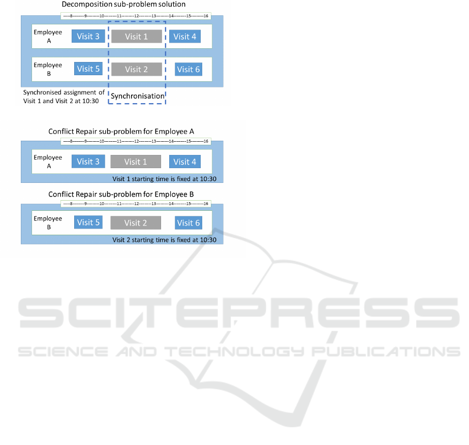
(a) Decomposition sub-problem solution
(b) Conflict Repair sub-problems
Figure 1: Time dependent modification example on syn-
chronised assignment. Sub-figure (a) shows solution from
solving a decomposition sub-problem. Sub-figure (b)
presents two conflict repair sub-problem solutions. As-
signed time from decomposition sub-problem solution on
visit with time-dependent activities (Visit 1 and Visit 2) are
carried on to the later stage of process. Time window of
Visit 1 and Visit 2 are fixed to the same value when prepar-
ing conflict repair sub-problem. Fixed starting time is en-
forced on Visit 1 and Visit 2 until both of them are cooper-
ated in final solution or the iterative process is terminated.
synchronisation and overlapping cases. Hence, these
constraints cannot be enforced by the conflict repair
directly because the method builds a sub-problem to
repair based on only one employee. Therefore, mod-
ification of the sub-problem to repair is necessary.
This is mainly to keep the layout of assignments when
time-dependent conditions are met.
Recall that the problem decomposition and sub-
problem solving stage involves solving sub-problems
in which visits share the same location and also
time-dependent visits are grouped in the same sub-
problem. Then, as defined by the MIP model, the so-
lution to a sub-problem satisfies all time-dependent
activities constraints. In order to keep the layout of
time-dependent activities, visits of sub-problems in
the conflict repair process require a fixed assigned
time for every time-dependent activities. The fixed
time is applied to time window α
i
= β
i
where i is a
time-dependent visit. Once the fixed time restriction
is enforced, it affects every iteration of the process.
Figure 1 shows an example of how the modifica-
tion works on a synchronisation constraint. With ref-
erence to the figure, suppose that visit 1 and visit 2
must be synchronised. Because visit 1 and visit 2
are time-dependent, they are grouped into the same
decomposition sub-problem. The decomposition sub-
problem is solved which gives paths for employee A
and employee B, as shown in Figure 1(a). From the
sub-figure, visit 1 and visit 2 are assigned to employee
A and employee B, respectively. Both visits have their
starting time set at 10:30. Suppose that both paths of
employee A and employee B need to be repaired. At
this stage, the time-dependent modification is applied.
It overrides the time window of both visits and sets
them to α
Visit1
= α
Visit2
= β
Visit1
= β
Visit2
= 10 : 30.
Here, we have two sub-problems to repair, presented
in Figure 1(b). Recall that a sub-problem to repair
is defined based on an employee who has conflicting
paths. Both sub-problems apply the new time win-
dow values forcing the start time of visit 1 and visit 2
to 10:30. The new time window is enforced until both
visits are assigned to the final solution or the iterative
process is terminated.
In the same way, the modification explained above
tackles the other types of time-dependent constraints.
The time-dependent visits are grouped in the same
sub-problem and the solution of this part satisfies
time-dependent activities constraints in the decompo-
sition step. The time-dependent modification also ap-
plies when the time-dependent visit needs to be re-
paired. The modification replaces the time window of
the visit by a fixed time given by the decomposition
step. Then, this modification ensures that a solution
that has gone through the conflict repair will satisfy
the time-dependent activities constraints.
4 EXPERIMENTS AND RESULTS
This section describes the experiments carried out to
compare the proposed RDCR method to the greedy
heuristic (GHI) in (Castillo-Salazar et al., 2015).
4.1 WSRP Instances Set
The RDCR method was applied to the set of WSRP
instances presented in (Castillo-Salazar et al., 2014;
Castillo-Salazar et al., 2015). Those problem in-
stances were generated by adapting several WSRP
from the literature. The instances are categorised in
four groups: Sec, Sol, HHC and Mov. The Sec group
contains instances from a security guards patrolling
scenario (Misir et al., 2011). The Sol group are in-
stances adapted from the Solomon dataset (Solomon,
1987). The HHC group are instances from a home
ICORES 2016 - 5th International Conference on Operations Research and Enterprise Systems
336

health care scenario (Rasmussen et al., 2012). Fi-
nally, the Mov group originates from instances of the
vehicle routing problem with time windows (Castro-
Gutierrez et al., 2011). The total number of instances
accumulated in these four groups is 374.
4.2 Overview of Greedy Heuristic GHI
A greedy constructive heuristic tailored for the WSRP
with time-dependent activities constraints was pro-
posed by (Castillo-Salazar et al., 2015). The algo-
rithm starts by sorting visits according to some crite-
ria such as visit duration, maximum finish time, max-
imum start time, etc. Then, it selects the first unas-
signed visit in the list and applies an assignment pro-
cess. For each visit c, the assignment process se-
lects all candidate employees who can undertake the
c (considering required skills and availability). If the
number of candidate employees is less than the num-
ber of employee required for visit c, this visit is left
unassigned. If visit c is assigned, visits that are de-
pendent on visit c are processed. These dependent
visits c
0
jump ahead in the assignment process and
are themselves processed in the same way (i.e. pro-
cessing other visits dependent on c
0
). The GHI stops
when the unallocated list is empty and then returns
the solution.
4.3 Computational Results
We applied the proposed RDCR method to the 374
instances and compared the solutions obtained to the
results reported for the greedy heuristic algorithm
(GHI) in (Castillo-Salazar et al., 2015).
First, the related-samples Wilcoxon Signed Rank
Test (Field, 2013) was applied to examine the differ-
ences between the two algorithms, GHI and RDCR.
The significant level of the statistical test was set at
α = 0.05. Results of this statistical test using SPSS
are shown in Table 4 showing that RDCR produced
209 better solutions out of the 374 instances. How-
ever, there was no statistical significant difference on
the solution quality between the two methods.
Figures 2 and 3 compare the number of best solu-
tions found by each of the two methods and the aver-
age relative gap to the best known solutions. In these
figures, results are grouped by dataset. Note that the
relative gap is calculated by ∆ = |z − z
b
|/|z
b
| where z
represents an objective value of a solution and z
b
is an
objective value of the best known solution. Regarding
the number of best solutions, RDCR produced better
results than GHI on three datasets: Sec, Sol and HHC.
Results also show that RDCR found lower values of
average relative gap on the same three datasets. On
Table 4: Statistical result from Related-Samples Wilcoxon
Signed Rank Test provided by SPSS.
Total N 374
# of (RDCR < GHI), RDCR is better than RDCR 209
# of (RDCR > GHI), GHI is better than GHI 165
Test Statistic 37,806
Standard Error 2,092
Standardized Test Statistic 1.311
Asymp. Sig. (2-sided test) .190
Sec Sol HHC
Mov
0
50
100
83
72
2
8
97
96
9
7
# Better solutions
GHI
RDCR
Figure 2: Number of best solutions obtained by GHI and
RDCR for each dataset.
the Mov dataset, GHI performed better in terms of
number of best solutions and average relative gap.
On datasets Sec and Sol, RDCR found slightly
better results than GHI as shown by the number of
best solutions and the average relative gap. In dataset
Sec, both RDCR and GHI gave 11% and 18% of av-
erage relative gap respectively. This indicates that
both algorithms provide good solution quality com-
pared to the best known solution. On the other hand,
both RDCR and GHI produced 1,216% and 1,561%
respectively for the average relative gap to the best
known solution in dataset Sol. This implies that both
algorithms failed to find solutions that are of competi-
tive quality to the best known solution, but both algo-
rithms are competitive between them. We can see that
instances in this Sol dataset are particularly difficult
as neither the GHI heuristic nor the RDCR decom-
position technique could produce solutions of similar
quality to the best known solution.
Sec Sol HHC
Mov
0
500
1,000
1,500
18
1,561
100
310
11
1,216
8.6
486
Relative gap (%)
GHI
RDCR
Figure 3: Average relative gap (relative to the best known
solution) obtained by GHI and RDCR. The lower the bar
the better, i.e. the closer to the average best known solution.
Mixed Integer Programming with Decomposition for Workforce Scheduling and Routing with Time-dependent Activities Constraints
337

0 10 20 30 40 50 60 70 80 90 100>100
100
200
300
400
Relative gap(%)
#Solutions
GHI
RDCR
Figure 4: Cumulative distribution of GHI and RDCR solu-
tion over the relative gap.
On dataset HHC, the average relative gap of
RDCR is much lower than the average gap of GHI.
The results show that RDCR has 8.67% relative gap
while GHI has 100.4%. For the HHC instances,
RDCR found the best known solution for 9 instances
and GHI found the best known solution for the other
2 instances. For these two instances, average relative
gap of RDCR is 47%. However, in the 9 best solutions
of RDCR, average gap of GHI is 109%. A closer look
at the Sol dataset showed that these instances have pri-
ority levels defined for the visits. It turns out that GHI
does not have sorting parameters to support such pri-
ority for visits because the algorithm sorting param-
eters focuses on the time and duration of visits. On
the other hand, RDCR implemented priority for visits
within the MIP model. This could be the reason that
explains the better results obtained by RDCR on this
particular dataset.
On dataset Mov, GHI gives better performance.
GHI delivers 8 better solutions (7 best known) from
15 instances while RDCR gives 7 better solutions (4
best known). The average relative gap of GHI is 310%
which is less than the 486% relative gap provided by
RDCR. There are 5 instances which best known solu-
tion is given by the mathematical solver. The average
relative gaps to the best known by GHI and RDCR
are 315% and 36% respectively. We found that the
decomposition method does not show good perfor-
mance on this particular Mov dataset, especially on
instances with more than 150 visits. The main rea-
son is that the solver cannot find optimal solutions to
the sub-problems within the given time limit. There-
fore, the size of sub-problems in these Mov instances
should be decreased to allow for the sub-problems to
be solved to optimally.
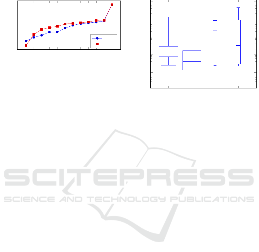
Figure 4 shows the cumulative distribution of
RDCR and GHI solution over the relative gap. It
shows the number of solutions which have a relative
gap to the best known less than the corresponding
value in the X-axis. Note that 0% relative gap refers
to the best known solution. GHI provides 115 best
known solutions which is better than RDCR which
Sec Sol HHC
Mov
10
0
10
1
10
2
10
3
10
4
Max GHI time
Seconds
Figure 5: Box and Whisker plots showing the distribution
of computational time in seconds spent by RCDR for each
group of instances. The wider the box the larger the number
of instances in the group. The orange straight line presents
the upper bound of the computational time spent by GHI
fixed to 1 second. The Y-axis is in logarithmic scale.
provides 84 best solutions. This is represented by
the two leftmost points in the figure. However, from
the value of 10% relative gap onwards, RDCR de-
livers larger number of solutions than GHI. Overall,
apart from the overall number of best known solu-
tions, RDCR provides higher number (or equal) of so-
lutions than GHI for different values of relative gap.
For example, if we set the solution acceptance rate at
50% relative gap, RDCR produces 236 solutions of
this quality while GHI produces 207. Hence, RDCR
delivers overall more solutions with acceptance rate
up to 100% gap to the best known.
Figure 5 shows the distribution of computational
time spent by the proposed RDCR method when solv-
ing the WSRP instances considered here. These re-
sults show that RDCR spends more computational
time on most of the HHC instances with an overall
average time spent on each instance of 2.4 minutes.
Note that the highest computational time observed in
these experiments is less than 74 minutes. On the
other hand, the computational time spent by GHI is
much less taking less than one second on each in-
stance. Therefore, GHI is clearly superior to RDCR
in terms of computational time.
5 CONCLUSION
This paper presented a decomposition method for
mixed integer programming to solve instances of the
workforce scheduling and routing problem (WSRP)
with time dependent activities constraints. The pro-
posed method is called Repeated Decomposition with
ICORES 2016 - 5th International Conference on Operations Research and Enterprise Systems
338

Conflict Repair (RDCR). First, the method decom-
poses a problem into several sub-problems. Then
each sub-problem is solved by an MIP solver. The so-
lutions to the sub-problems usually include conflict-
ing paths, i.e. two or more different sequences of vis-
its but assigned to the same employee. These conflict-
ing paths are tackled with a conflict repair process.
Then, time-dependent activities modification is ap-
plied to tackle time-dependent activities constraints.
This process maintains the layout of a solution so that
a time-dependent activities constraint is valid.
The proposed RDCR approach is applied to solve
four WSRP scenarios which provide a total of 374
problem instances. The experimental results showed
that RDCR was able to find better solutions than
the GHI heuristic for 209 out of the 374 instances.
However, the statistical test showed that RDCR does
not perform significantly different to the deterministic
greedy heuristic (GHI). RDCR showed better perfor-
mance on three out of four datasets.
The computational time required to solve a prob-
lem instance with RDCR ranged from less than a sec-
ond to 74 minutes. The average computational time
was under 3 minutes. Overall, the proposed RDCR
with time-dependent modification is able to effec-
tively solve WSRP instances with time-dependent ac-
tivities constraints. The method found competitive
feasible solutions to every instance and within reason-
able computational time.
Our future work is towards improving the compu-
tational time of the proposed RDCR approach. Such
improvement might be achieved by applying different
methods to partition the set of visits or by using more
effective workforce selection rules. Also, determining
the right sub-problem size could be interesting as it
could help to balance solution quality and time spent
on computation.
ACKNOWLEDGEMENTS
We are grateful for access to the University of Not-
tingham High Performance Computing Facility. Also,
the first author thanks the DPST Thailand for partial
financial support of this research.
REFERENCES
Akjiratikarl, C., Yenradee, P., and Drake, P. R. (2007).
PSO-based algorithm for home care worker schedul-
ing in the UK. Computers & Industrial Engineering,
53(4):559–583.
Castillo-Salazar, J. A., Landa-Silva, D., and Qu, R. (2014).
Workforce scheduling and routing problems: litera-
ture survey and computational study. Annals of Oper-
ations Research, doi:10.1007/s10479-014-1687-2.
Castillo-Salazar, J. A., Landa-Silva, D., and Qu, R. (2015).
A greedy heuristic for workforce scheduling and rout-
ing with time-dependent activities constraints. In Pro-
ceedings of the 4th International Conference on Op-
erations Research and Enterprise Systems (ICORES
2015).
Castro-Gutierrez, J., Landa-Silva, D., and Moreno, P. J.
(2011). Nature of real-world multi-objective vehi-
cle routing with evolutionary algorithms. In Systems,
Man, and Cybernetics (SMC), 2011 IEEE Interna-
tional Conference on, pages 257–264.
Cordeau, J.-F., Laporte, G., Pasin, F., and Ropke, S. (2010).
Scheduling technicians and tasks in a telecommuni-
cations company. Journal of Scheduling, 13(4):393–
409.
Field, A. (2013). Discovering Statistics Using IBM SPSS
Statistics. SAGE Publication Ltd, London, UK, 4 edi-
tion.
Laesanklang, W., Landa-Silva, D., and Castillo-Salazar,
J. A. (2015). Mixed integer programming with decom-
position to solve a workforce scheduling and routing
problem. In Proceedings of the 4th International Con-
ference on Operations Research and Enterprise Sys-
tems (ICORES 2015), pages 283–293.
Mankowska, D., Meisel, F., and Bierwirth, C. (2014). The
home health care routing and scheduling problem with
interdependent services. Health Care Management
Science, 17(1):15–30.
Misir, M., Smet, P., Verbeeck, K., and Vanden Berghe, G.
(2011). Security personnel routing and rostering: a
hyper-heuristic approach. In Proceedings of the 3rd
International Conference on Applied Operational Re-
search, ICAOR2011, Istanbul, Turkey, pages 193–205.
Rasmussen, M. S., Justesen, T., Dohn, A., and Larsen, J.
(2012). The home care crew scheduling problem:
Preference-based visit clustering and temporal depen-
dencies. European Journal of Operational Research,
219(3):598–610.
Reimann, M., Doerner, K., and Hartl, R. F. (2004). D-
Ants: Savings based ants divide and conquer the ve-
hicle routing problem. Computers & Operations Re-
search, 31(4):563 – 591.
Solomon, M. M. (1987). Algorithms for the vehicle rout-
ing and scheduling problem with time window con-
straints. Operations Research, 35(2).
Xu, J. and Chiu, S. (2001). Effective heuristic procedures
for a field technician scheduling problem. Journal of
Heuristics, 7(5):495–509.
Mixed Integer Programming with Decomposition for Workforce Scheduling and Routing with Time-dependent Activities Constraints
339