A Pareto Front Approach for Feature Selection

Enguerran Grandchamp

, Mohamed Abadi

and Olivier Alata

Laboratoire LAMIA, Université des Antilles, Campus de Fouillole, 97157 Pointe-à-Pitre Guadeloupe, France

Institut XLIM-SIC, UMR CNRS 6172, Université de Poitiers, BP 30179, 8962 Futuroscope-Chasseneuil Cedex, France

Lab. Hubert Curien, UMR CNRS 5516, Univ. Jean Monnet Saint-Etienne, Univ. Lyon, 42000, Saint-Etienne, France

Keywords: Hybrid Feature Selection, Mutual Information, Multiobjective Optimization, Pareto Front, Classification.

Abstract: This article deals with the multi-objective aspect of an hybrid algorithm that we propose to solve the feature

subset selection problem. The hybrid aspect is due to the sequence of a filter and a wrapper method. The filter

method reduces the exploration space by keeping subsets having good internal properties and the wrapper

method chooses among the remaining subsets with a classification performances criterion. In the filter step,

the subsets are evaluated in a multi-objective way to ensure diversity within the subsets. The evaluation is

based on the mutual information to estimate the dependency between features and classes and the redundancy

between features within the same subset. We kept the non-dominated (Pareto optimal) subsets for the second

step. In the wrapper step, the selection is made according to the stability of the subsets regarding classification

performances during learning stage on a set of classifiers to avoid the specialization of the selected subsets

for a given classifiers. The proposed hybrid approach is experimented on a variety of reference data sets and

compared to the classical feature selection methods FSDD and mRMR. The resulting algorithm outperforms

these algorithms.

1 INTRODUCTION

Feature Selection (FS) is an active topic of interest. A

large number of algorithms have been proposed. The

basic idea is to select a subset from a large set of

features. FS is a branch of the Dimension Reduction

problem (Hilario, 2008). FS is an important task in

many fields such as text characterization, image

research, bioinformatics, color image processing,

data mining, etc. The aim is to select relevant features

for knowledge interpretation or representation,

computation time reduction and overall improvement

in performance (such as classification accuracy).

The relevancy of the features can have different

definitions depending on the application: in

knowledge interpretation or representation, the size

reduction and the semantic and/or the diversity of the

selected features are important in order to keep in a

lower dimension the topological structure of the

information; for classification applications,

relevancy is directly linked to a good rate in learning

or classification; in protein biomarkers identification,

the reduction of the feature subset size and its stability

when applying different learning sets are more

important than classification performances. The

relevancy is linked to the quality, the complexity, the

diversity or the performance of the feature subset.

Different approaches have been developed to

select a subset of features. They differ by their

research method to explore the subsets, their criterion

for comparing and ranking them and their selection

process.

We design a hybrid method to combine the

advantages of both filter and wrapper approaches: a

fast (filter) way to select diversified subsets (multi-

objective) having good internal properties (filter) and

a final selection based on performances (wrapper).

The stability criterion avoid specializing the subsets

to a given classifiers.

After a general presentation of the main

exploration methods, the fitness functions and

selection processes are presented in section 2. Section

3 presents the multi-objective principle. Then in

section 4, we present the hybrid method and the

criterions. In section 5, some formalism is given

concerning the criterion, the non-domination

principle and the algorithm. The algorithm is given in

section 6. The experiments on benchmarking

database, classification and segmentation

applications are given in section 7. Finally, section 8

gives conclusions and perspectives of the work.

334

Grandchamp, E., Abadi, M. and Alata, O.

A Pareto Front Approach for Feature Selection.

DOI: 10.5220/0005752603340342

In Proceedings of the 5th International Conference on Pattern Recognition Applications and Methods (ICPRAM 2016), pages 334-342

ISBN: 978-989-758-173-1

2 THE FEATURE SELECTION

PROBLEM

Many papers have been published on the modeling

and the description (Somol, 2010) of feature selection

problem. We summarize the main ideas implemented

in the different feature selection approaches.

Categorization is done according to

Exploration methods (Sun, 2010) :

• Greedy methods based on sequential approaches

such as Sequential Forward Selection (SFS) and

Sequential Backward Selection (SBS).

• Sequential Forward Floating Selection (SFFS)

and Sequential Backward Floating Selection

(SBFS).

• Genetic Algorithms (GA)

Fitness functions:

• A quality measure evaluated on each features

separately: Dependency, entropy, relief-f,

distance measures, statistical measures and more

recently probabilistic measures based on the

estimation of Mutual Information (Peng, 2005);

or directly on the subset: correlation,

redundancy, Information Criteria, for example.

• A performance measure: the good classification

rate or error rate during the learning step.

• A complexity measure: the cardinality of the

subset, the complexity of the classifiers.

Selection processes:

• A single candidate selection for sequential

approaches: maximization (classification rate,

relevancy, etc.) or minimization (error rate,

correlation, etc.) of the criterion.

• Multiple candidates for evolutionary approaches

The main used evaluation is based on their

performances in a classification context.

These different approaches lead to the separation of

the methods in four families based on how to compare

and rank the subsets:

• Wrapper methods use a machine learning

algorithms during the exploration step to

evaluate the candidate’s subsets and the

corresponding classifier during the evaluation of

the returned solution (test stage). It often gives

the best performances but it is time consuming

because of the training step on classifiers.

• Filter methods use an independent criterion to

measure the quality of the feature subsets. These

methods are the most popular because they

considerably reduce the computation time.

• Embedded methods try to combine the

advantages of both approaches. Nevertheless, the

computation time still remain important.

• Hybrid methods use a sequence of Filter and

Wrapper methods (Peng, 2005).

More details are given in the previous references and

particularly in (Hilario, 2008) and (Somol, 2010)

which are surveys of methods.

3 A MULTI OBJECTIVE

APPROACH

Most of the time the exploration methods deal with a

single criterion. However the use of only one

characteristic to rank and select the subsets is

insufficient in many cases. Authors then defined

combinations of several criterions to integrate quality

and performance. In practice, defining a combination

of criterions is not an easy task. It depends on the

application and often requires parameters to balance

the different parts of the criterion. These criterions

generally have opposite behaviors because increasing

the performances often requires adding features

which increase complexity.

In order to bypass this drawback, a multi-

objective approach has been adopted in some studies

(Hasan, 2010). A multi-objective approach try to

simultaneously optimize several fitness functions

during the exploration. However the criterions often

have opposite behaviors leading to a set of non-

dominated solutions called the Pareto set.

For the FS problem, the different approaches, deal

with wrapper methods using GA as exploration

method with a simple binary encoding and standard

crossover and mutation. One of the objective is the

cardinality of the subset and the other one a

classification rate or error rate.

4 THE PROPOSED HYBRID

APPROACH

4.1 Filter and Wrapper Combination

Hybrid methods are proposed in the literature (Cantu-

Paz, 2004), (Peng, 2005), but the main objective of

these works is to reduce the computation time. Indeed

the criterion used in the wrapper step is the classifier

performance in a mono-objective approach. The filter

method is used to reduce the exploration space in a

very high dimensional data set by evaluating the

quality of the features in a mono-objective way:

Kullback-Leiber distance between histograms of

feature values; mRMR criterion; the relief criterion

and; the relative certainty gain.

A Pareto Front Approach for Feature Selection

335

The way to select the subsets for the wrapper step

represents the main differences between the

approaches. In (Cantu-Paz, 2004) they select the

features by fixing a threshold on the Kullback-Leiber

distance; In (Peng, 2005), they keep subsets having a

classification error under a given threshold.

As the number of features is reduced by the filter

step, the wrapper step manages the retained features

by the mean of a classical GA, or sequential forward

and backward search with a classification accuracy

criterion.

We propose a hybrid method by combining the

Filter and Wrapper methods in two sequential steps.

This approach improves the lack of diversity of the

solutions returned by standard algorithms and reduces

the dependency between subsets and classifiers. The

computation time remains acceptable thanks to the

use of a fast filter approach and a controlled

exploration of Pareto solutions during the first step.

These procedures coupled with a multi-objective

approach with two quality objectives allow keeping

diversity. All the selected subsets using the Pareto

front are evaluated during the wrapper step.

We prefer a stability criterion to select the final

subsets instead of raw performances regarding one

classifier, in order to keep performances and

independency between subsets and classifiers.

Indeed, we are looking for diversified subsets in

the filter step in order to have different kinds of

solutions to be evaluated during the wrapper step to

increase the probability to reach stable ones. In this

way, the building of the Pareto front seems to be the

more appropriate choice.

4.2 Criterion and Diversity

The second stage of some previous approaches

maintains a kind of diversity by the crossover step and

the mutation step of a GA. On the other hand, the

selection of the first pool of features by the filter step

is done using a single criterion which restricts the

explored subsets. Indeed, the evaluation of the subsets

is done in a single way which leads to reject subsets

having good properties according to another criterion.

This is particularly the case for single criterions

which are composed of multiple parts (mRMR for

example, composed of Redundancy and Relevance).

In this context, solution having very low redundancy

or very high relevance could be rejected by the

selection process if the resulting aggregation function

has a low evaluation. To increase the diversity of the

selected subsets our filter step explores the space in a

multi-objective way with two quality objectives and

a complexity objective.

The evaluation of the quality is based on the Mutual

Information (MI) to separately measure the

Dependency (D) and Redundancy (R) of the subsets.

The theoretical interest for Mutual Information has

been proved in (Peng, 2005). These two criterions

measure both the individual quality of the selected

features and the quality of the subset. The separate

evaluation of these two measures (contrary to (Peng,

2005)) is important because a relevant subset is not

necessarily a subset containing only significant

attributes taken alone. Indeed the relevance of a

subset may be due to combinations of features.

5 CRITERIONS

The criterions are based on the mutual information

which is considered to be a good indicator to study

the dependency between a feature and the

classification and the redundancy between random

features.

Mutual Information

Let  and  be two random variables with discrete

probability laws. The Mutual Information (MI)



(

;

)

is defined by 

(



)

, 

(



)

and 

(

,

)



(

;

)

=

(

,

)

∙log



(

,

)



(



)

∙

(



)

∈



∈



(1)

with Ω

and Ω

the sample spaces of X and Y

respectively.

When  and  are dependent, 

(

;

)

is high.



(

;

)

is equal to zero when  and  are

independent.

Selection criterion definition

For each subset of features, we define the

relevance expressed by the Dependency (D) which is

the average MI between the variables of S (X

) taken

separately and the class of the samples modeled by a

discrete random variable called c with sample space

equal to the class labels:









∑



(





;

)





∈

(2)



(





;

)

represents the MI between a variable and the

classes. It translates how X

is useful to describe the

classes.

The Dependency has to be maximized. However

in order to have a homogenous expression of the

objective we prefer to express the opposite of the

Dependency (-D) to minimize each criterion.

The feature selection using only  is not optimal

because of redundancy between the variables.

ICPRAM 2016 - International Conference on Pattern Recognition Applications and Methods

336

Different ways exist to measure the redundancy and

we use the one expressed in (Peng, 2005). It is based

on the computation of the average MI between two

variables 



;





,,⋯,

belonging to the same

subset  having  variables.











∑





;









,



∈

(3)

The redundancy must be minimized.

6 HYBRID AND

MULTIOBJECTIVE

ALGORITHM

6.1 Principle

The novelty of our approach is that previous

criterions are treated separately contrary to (Peng,

2005) and (Al-Ani, 2002) where criterions are

combined to produce the mRMR (minimal-

redondance-maximale-pertinence) criterions (ex.

max



(





−



)

or max



(





/



)

). These mono-objective

criterions didn’t ensure the simultaneous

convergence of criterions

(

)

and

(

)

to their optimal

value but lead to a trade-off between them.

We also keep the subset cardinality (L) which must

be minimized as a third criterion.

The goal of a multi-objective optimization is to

improve several criterions. When these criterions

have opposite behaviors considering the research of a

solution, we necessarily have to degrade at least one

criterion to improve another one. This leads to

different kind of solutions which are not necessarily

comparable. If we don’t want to make a choice

between solutions we must keep all solutions being

better than any others on at least one criterion. This

leads to the notion of domination which is essential to

ensure diversity in the final sets.

Without loss of generality, we illustrate this notion

in our particular case.

Following the previous section, each subset is

evaluated with three values (



,



,



)=(−D,R,L).

• A subset S dominates a subset S

according to 



if 



(

)

<



(



)

. i=1, 2, or 3

• A subset S dominates a subset S

if ∀



(

)

≤





(



)

and ∃|



(

)

<



(





)

• A subset S is not dominated if

∄



|



dominatesS (∄



|∀



(





)

≤





(

)

, ∃



(





)

<



(

)

).

• The set of all non dominated subsets is called the

Pareto set.

The third criterion, which represents the

complexity of the subset through its cardinality,

allows keeping subsets with different size (for low

number of features the redundancy may be better and

for high number of features the dependency may be

better). Nevertheless, even if we have one Pareto

front for each possible subset size, there is no

certainty to obtain at least one subset for each possible

size. This could be an inconvenient for some

applications. In such condition, the exploration step

can deal with only the quality criterions and each

intermediate Pareto front (corresponding to a specific

size) could be kept. This approach called Multi Pareto

Front (MF) is detailed in the next paragraph.

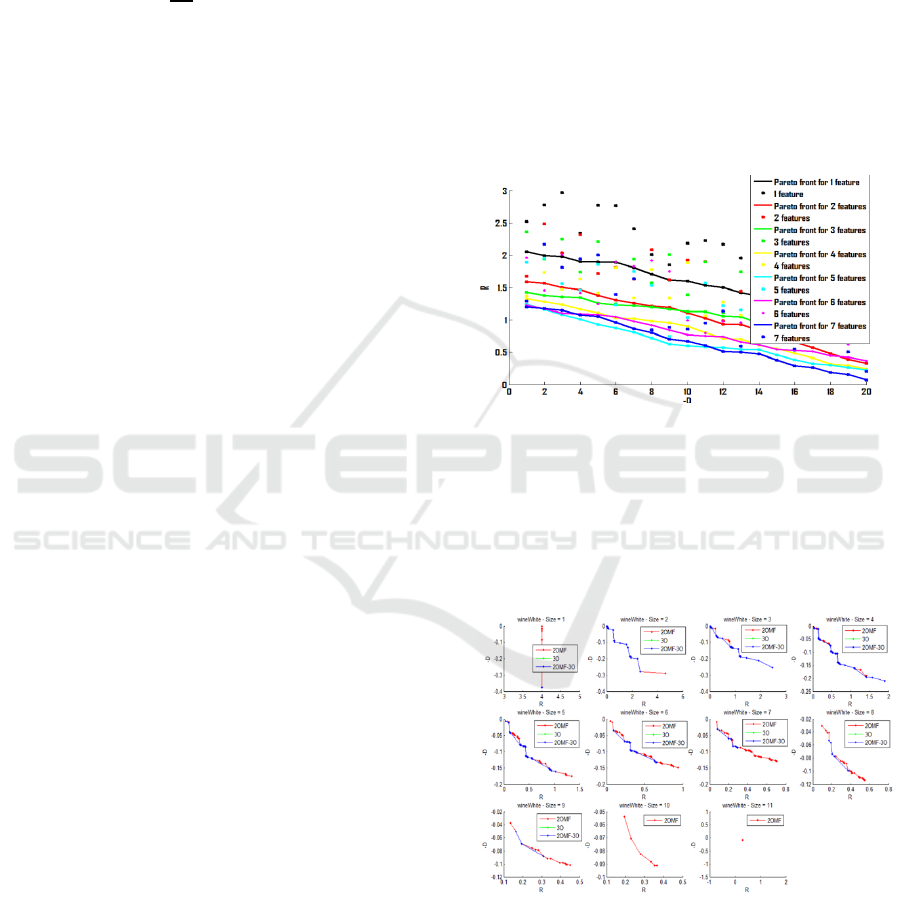
Figure 1: Pareto front evolution principle.

Figure 1 illustrate the evolution of the Pareto front

projected in (-D,R) space. As the number of features

increases the solutions in the Pareto front tend to

decrease –D and R values. Figure 2 shows the same

with in a real case using wineWhite database of the

UCI.

Figure 2: Pareto front evolution for wineWhite UCI

database.

6.2 Filter Step: Multiobjective

Exploration

For any optimization problem, a unique Pareto set

exists for a given data set and the considered

A Pareto Front Approach for Feature Selection

337

criterions. In a muti-objective context, an exhaustive

search, or an algorithm having asymptotic

convergence properties such as Genetic algorithm, is

classically required to find this set. Both are time

consuming and sometimes too slow to reach the

optimal Pareto set in a reasonable time. In practice,

people build a sub-optimal Pareto front which is the

Pareto front computed over the visited solutions. One

of the main qualities of a search method is then its

ability to provide solutions close to the ones of the

optimal Pareto front. Our filter search method joins

this way and has been developed to approach the

building of the optimal Pareto front.

The filter step uses a sequential forward search to

explore the subset space adopting the following

algorithm:

1. Let =







 ∈ [1,]} be the complete set

2. We start with all possible pairs of

features 



=



,



 ∈

[

1,

]

,∈

[

1,

]

,≠}.

3. Each subset S is evaluated with (-D(S),

R(S)) criterions and the non-dominated

subsets (



) are preserved. 



is the

Pareto front at iteration 2 (



=



4. At iteration k, 



 is the non dominated

subsets of size k (k>2) and 



is the

global Pareto Front (



⋃









5. We build V

k+1

by adding to 



one new

feature taken within the remaining

features: 





(

∪



 ∈ 



,



∈\}.

Each subset S in V

k+1

is then evaluated

with (-D(S), R(S)).

6. We build ND

k+1

by retaining the non

dominated subsets of size k+1 within 



.

We note that ND

k+1

⊆



. This step is

required because some subsets of 



can

be dominated by ones of 



(opposite is

impossible because each subset in 



is

greater than the ones in 



7. The algorithm ends if k=M.

This algorithm is called two Objectives Multi-

Front Algorithm (2OMF) and the returned set of

subsets is 



⋃









We can note that



⊆ 



. Indeed, subsets of





couldn’t dominate subsets of 



because these

last ones have a lower size: ∀



∈



,

(





)

≤

,∀



∈



,

(





)

=+1.

6.3 Wrapper Step: Stability Criterion

The wrapper step is used to rank the selected subsets

and to select a subset considering the application. For

this step, the exploration space has been sufficiently

reduced during the filter step to allow an exhaustive

evaluation of the remaining subsets ND

. A large

majority of wrapper approaches deals with Feature

Selection in terms of performances regarding a

classifier, but few studies select subsets for their

stability. Nevertheless, the stability is a topic of

interest in studies dealing with high dimensional data

and a small number of samples (Hilario, 2008).

Moreover, wrapper methods can lead to good

classification accuracy for a specific classifier but

with poor generalization properties (Kalousis, 2007),

(Peng, 2005) (i.e. over-fitting for one classifier and

low performances for another one).

The stability is defined by (Somol, 2010) as being

the quality of a subset to have the same performances

with different training sets. Different stability indices

can be used such as Hamming distance, correlation

coefficients, Tanimoto distance, consistency index

(simple, weighted or relative weighted) and Shannon

entropy. In (Kuncheva, 2007) and, the stability is

measured by running a wrapper scheme several times

with a unique classifier and different learning sets (no

cross-validation). The stability is based on an

evaluation of the similarity between subsets returned

by different runs. If the index is high the subset is

selected. Otherwise the selection is based on the

classification rate evaluation.

In this paper, we investigate another kind of

stability between different classifiers (each trained

and evaluated with a cross-validation process).

According to this kind of stability has been neglected

in the literature. A subset is stable regarding

classifiers if the performances obtained with different

classifiers are close. The easiest way to compute the

stability of a subset is to compute the amplitude of the

classification rates obtained with several classifiers

K-Nearest Neighbor (KNN), Linear Discriminant

Analysis (LDA), Mahalanobis (Mah), Naive Bayes

(NB), Simple Vector Machine (SVM) and

Probabilistic Neural Network (PNN):

() =max

∈





(S)

}

−min

∈





(S)

}

(4)

Where S is the subset, Cl a set of classifiers and R



(S)

the classification rate obtained with the classifier c

applied on the subset S.

Finally, we identify the stable and successful

subsets. Therefore, the selection of the interesting

subsets is done in a two objectives way by

maximizing the mean classification rate (()) and

by minimizing the amplitude (()).

()=mean

∈





(S)

}

(5)

7 RESULTS

In a first step we present the results obtained with the

2OMF algorithm. In a second step we compare the

ICPRAM 2016 - International Conference on Pattern Recognition Applications and Methods

338

2OMF method with two other existing feature

selection methods: mRMR (Peng, 2005) and FSDD

(Liang, 2008). Both are using filter criterions to select

the features and then they evaluate the unique

returned solution using classifiers. We choose mRMR

method because it uses the same criterions as 2OMF

but in a mono-objective way. We choose FSDD

because it is a fast algorithm which converges to the

optimal solution regarding a distance criterion. In

both cases, it is interesting to project the solutions

obtained with different filter steps in the space

(performance, stability) of the wrapper step and to

compare them with our pool of solutions. The

comparison is done by means of the size and the

stability of the subsets returned by each method and

also the computational time of each method.

Each step uses UCI databases for validation and

more particularly iris, TAE, abalone,

PimaIndiansDiabetes, wineRed, wineWhite, wine,

imgSeg, ionosphere and landSat databases containing

4, 5, 7, 8, 11, 11, 13, 18, 34 and 36 features

respectively. Figure 3 to 5 present some of the

obtained results. The stability is computed after

applying KNN, LDA, Mah, NB, and PNN classifiers.

7.1 2OMF Method Analysis

We analyse more precisely the results of the 2OMF

algorithm after the second step of the algorithm. This

step is based on the wrapper approach which sorts

and then selects among the retained subsets during the

filter step. We recall that the used criterion is the

stability (in a two objectives way) when different

classifiers are applied. In this space (mean rate,

amplitude) we compute a new Pareto front composed

of several solutions and we focus on them to select

the most interesting ones.

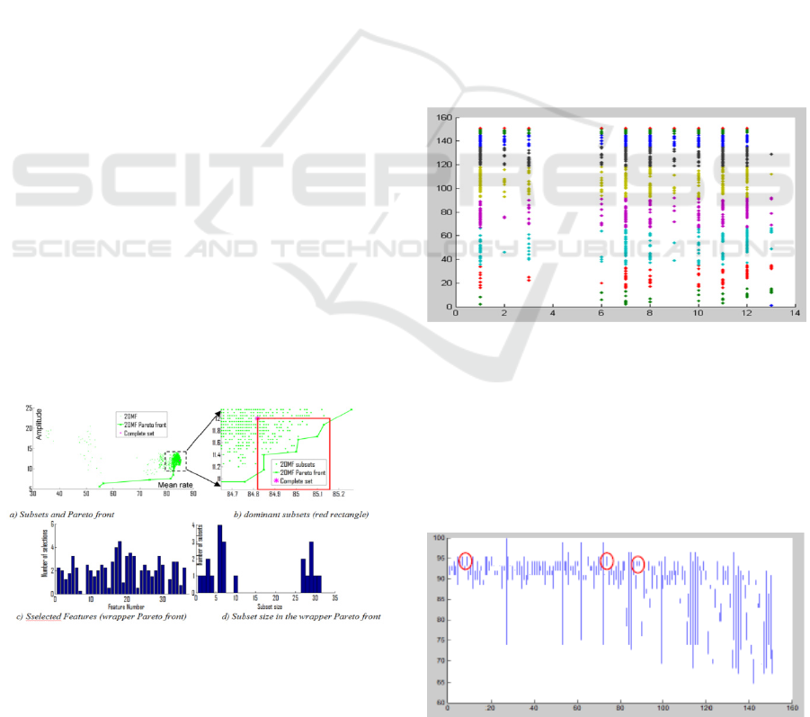
Figure 3: Stability analysis for landSat database.

The Figure 3 displays information about the

stability of the selected subsets after filter step (green

points) for landSat database. As showed in Figure 3

b) (which is a zoomed part of the Figure 3 a) ), a lot

of subsets dominates the complete set (purple star in

the figure) even if they are not in the Pareto front:

these subsets are within the red rectangle. All of these

subsets have higher mean classification rate and

lower amplitude than the complete set. They can also

be interesting because some of them have lower

number of features than the one in the Pareto Front

and a quite good classification stability as it is better

than the complete set stability. For the studied

database, there are 21 subsets in the front (6

dominating complete set) and 73 subsets that

dominate the complete set.

Figure 3 c) shows the histogram of the selected

features computed using all subsets of the 2OMF

wrapper Pareto Front. We note that quite every

features are represented. In the same way Figure 3 d)

gives the repartition of the size of the Pareto subsets

in order to illustrate the diversity of the solutions.

Landsat database is composed of 36 features and

some of the subsets in the Pareto front are composed

of less than 10 features. A further analysis of the

subset sizes is given in the next section.

Figure 4: Wine features used.

Figure 4 shows the features used by the different

Pareto solutions for the wine database. We remark

that some features are not present (4 and 5) or

underrepresented (2, 9) in the Pareto front and some

are overrepresented (1, 7, 8, 11, 12). This suggests a

individual quality evaluation of the features which

could be studied later.

Figure 5: Wine Pareto front wrapper stability.

A Pareto Front Approach for Feature Selection

339

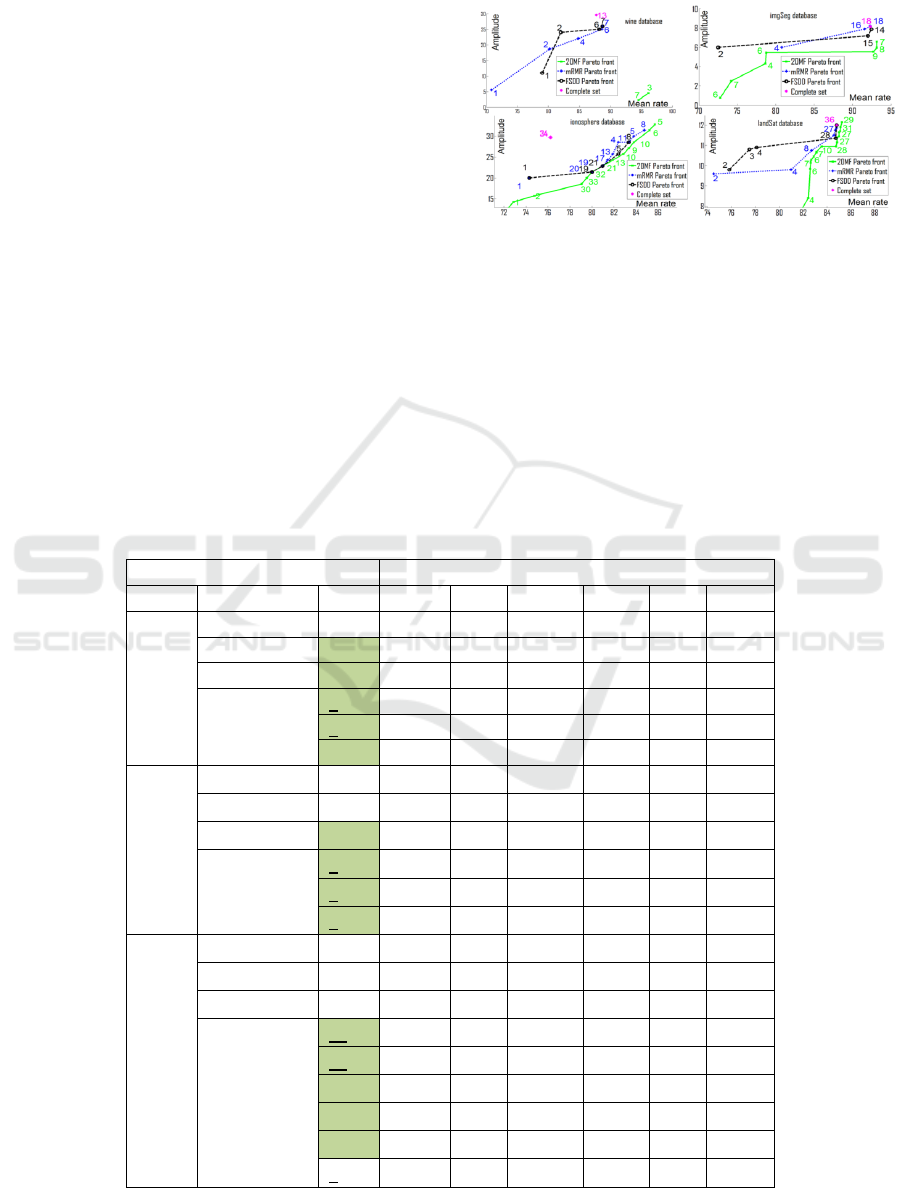
Figure 5. shows the min and max good classification

rate after the wrapper step for each Pareto front

solution for wine database. We remark a great

diversity both in terms of good classification rate than

in terms of standard deviation. In this view we are

looking for solutions having a high classification rate

and a low standard deviation (examples are given

within the red circles).

7.2 Comparison between 2OMF,

mRMR and FSDD

We compare our algorithm with two well-known

feature selection methods: mRMR and FSDD. Figure

6 displays the visited subsets using mRMR algorithm

(blue) with their corresponding Pareto front (blue

line) and using FSDD algorithm (black) with their

corresponding Pareto front (black line). We observe

that these subsets are not Pareto optimal when

compared to the 2OMF subsets (green points).

Moreover, few of them dominate the complete subset.

The same observation can be done for most of the

databases. Indeed, in few databases we observe an

mRMR subset that dominates the complete subset. A

subset of mRMR and a subset of FSDD fall into the

Pareto set only for TAE database and for iris.

Figure 6: Comparison of the stability Pareto Fronts for

2OMF (green), mRMR (blue) and FSDD (black)

algorithms.

The size of the corresponding subsets is also

displayed near the subset as well as the complete set

(purple star). We can observe that the subset size

follows high variations: between 2 and 33 for the

2OMF Pareto front for ionosphere database and

between 4 and 29 for the 2OMF Pareto front of the

landSat database for example. The mean

classification rate is also varying in a wide range: for

Table 1: Good classification rate and stability of interesting subsets (Bold faces indicate the best result(s)).

Classifiers Rate

Db Method Size Mean Var KNN Mah NB PNN

Wine

Fill set 13 87.7 29.5 70.4 92.0 96.6 79.5

Best mRMR 6 88.63 25.0 73.8 97.7 97.7 75

Best FSDD 6 88.18 25.0 73.8 97.7 95.4 75.0

2OMF

3 96.2 4.5 97.7 96.6 97.7 95.4

7 94.5 2.2 95.5 93.2 95.5 95.5

2 94.3 5.6 96.6 94.3 95.5 94.3

imgSeg

Full set 18 92.3 8.2 95.5 NA 87.3 95.3

Best mRMR 16 91.57 7.9 94.9 NA 87 94

Best FSDD 14 92.46 7.87 95.3 NA 87.5 95.4

2OMF

7 93.2 6.5 96.1 NA 89.5 96.0

8 93.1 5.9 96.0 NA 90.0 95.6

9 92.7 5.5 95.2 NA 89.8 95.4

landSat

Full set 36 84.8 12 89.4 81.6 78.5 90.5

Best mRMR 27 84.58 11.5 89.8 80.1 79.2 90.7

Best FSDD 28 84.73 11.3 89.7 80.8 79.2 90.5

2OMF

29 85.0 11.4 89.8 82.1 78.9 90.3

31 85.1 11.9 89.6 83.0 78.7 90.6

27 84.85 11.1 89.9 81.4 79.2 90.3

25 84.9 11.9 89.3 82.7 78.7 90.6

26 84.8 11.7 89.6 82.3 78.6 90.6

7 83.13 10.7 84.9 83.1 72.2 87.9

ICPRAM 2016 - International Conference on Pattern Recognition Applications and Methods

340

ionosphere database the mean rate is about 75.5% for

a two features subset, 86% for a 5 features subset and

84% for a 10 features subset; for the landSat database

the mean rate is about 82.5% for a 4 features subset

and 85.5% for a 28 features subset.

We now focus on the good classification rate

obtained for some interesting subsets. The table 1.

shows subsets obtained with 2OMF, mRMR and

FSDD methods. Information about the Pareto

optimality is also given (Underlined size in table). In

addition to this, we present whether a subset

dominates the complete set (Green background color

in table). The mRMR and FSDD subsets are chosen

among the visited ones according to their mean rate

value.

All the displayed subsets obtained with the 2OMF

method are interesting because they have a low

number of features and a better stability than the

complete set. Nevertheless, some subsets have lowest

number of features and others highest classification

rates. For example, for the wine database, a subset

with two features (features 2 and 7) have a higher

mean rate and a lower amplitude than the complete

set having 13 features. Moreover, it has a higher

classification rates for 4 classifiers over 5. In the same

way, for imgSeg database the number of features is

divided by 2 with the 2OMF method.

Let us consider now the methods from the

literature. For landSat database none of the visited

subsets dominate the complete set for both mRMR

and FSDD. Moreover, stable and successful subsets

obtained with FSDD have a higher number of features

than the ones obtained with 2OMF. Only one stable

subset having low number of features is obtained with

mRMR (8 features). However, it is dominated by the

subset returned by 2OMF which has seven features

(last line in the table). We always found a subset

among 2OMF subsets having a lower number of

features, a higher classification mean rate and a lower

classification amplitude than the best subsets returned

by mRMR and FSD.

8 CONCLUSION

This paper presents a two steps algorithm for feature

selection and studies its multi-objective aspect. The

algorithm begins with a filter step to quickly select a

first pool of subsets in a Multi-Objectives and Multi-

Fronts way (2OMF). The subsets are evaluated using

the Dependency (D) and the Redundancy (R) of the

features. Then a second step based on a wrapper

approach is applied to measure the performances of

the subsets regarding several classifiers (KNN, LDA,

Mah, NB, PNN). Then the selection of the interesting

subsets is performed using the stability of the subsets

which is evaluated with the mean and amplitude of

the classification rates. From our experimentations, it

is observed that the interesting subsets dominate the

complete set regarding both objectives. The use of the

stability to select the subsets leads to robust results

which are very interesting for some applications such

as in biology where the stability of the subsets is more

important than its raw classification rate. The

wrapper step is required because some subsets of the

filter Pareto front could have a higher classification

rate than the complete set for a given classifiers but

not for another one. A selection of features only based

on a filter method does not ensure that the selected

subset will improve classification rates for a large set

of classifiers.

The results are very convincing for all tested

databases. The subsets obtained after applying our

algorithm have lower number of features and better

classification performances compare to the complete

set of features. Moreover, the diversity of the final

pool of subsets allows selecting a subset adapted to a

specific application (good classification expected or

reduction of a high number of features). We also

compared the proposed algorithm with two feature-

selection methods (mRMR and FSDD). It is observed

that our method outperforms the other tested methods

in almost all cases.

REFERENCES

A. Al-Ani, M. Deriche, and J. Chebil, "A new mutual

information based measure for feature selection,"

Intelligent Data Analysis, vol. 7, no. 1, pp. 43-57, 2003.

E. Cantu-Paz, "Feature Subset Selection,Class

Separability, and Genetic Algorithms," in Genetic and

Evolutionary Computation, 2004, pp. 959-970.

K. Deb, Multi-Objective Optimization Using Evolutionary

Algorithms.: John Wiley and Sons, Chichester, 2001.

C. Emmanouilidis, A. Hunter, and J. MacIntyre, "A

Multiobjective Evolutionary Setting for Feature

Selection and a Commonality-Based Crossover

Operator," in Congress on Evolutionary Computation,

California, July 2000, pp. 309-316.

B.A.S. Hasan, J.Q. Gan, and Z. Qingfu, "Multi-objective

evolutionary methods for channel selection in Brain-

Computer Interfaces: Some preliminary experimental

results," in IEEE Congress Evolutionary Computation,

Barcelona, Spain, July 2010, pp. 1-6.

M. Hilario and A. Kalousis, "Approaches to dimensionality

reduction in proteomic biomarker studies," Briefings in

Bioinformatics, vol. 9, no. 2, pp. 102-118, 2008.

A. Kalousis, J. Prados, and M. Hilario, "Stability of feature

selection algorithms: A study on high-dimensional

A Pareto Front Approach for Feature Selection

341

spaces," Knowledge and Information Systems, vol. 12,

no. 1, pp. 95-116, 2007.

I. Kononenko, "Estimating attributes: Analysis and

extensions of RELIEF," in ECML-94, 1994, pp. 171-

182.

L.I. Kuncheva, "A stability index for feature selection," in

Proceedings of the 25th conference on Proceedings of

the 25th IASTED International Multi-Conference:

artificial intelligence and applications, Innsbruck,

Austria, February 2007, pp. 390-395.

N. Kwak and C.H. Choi, "Input Feature Selection by

Mutual Information Based on Parzen Window," IEEE

Trans. Pattern Anal. Mach. Intell, vol. 24, no. 12, pp.

1667-1671, 2002.

J. Liang, S. Yang, and A-C. Winstanley, "Invariant optimal

feature selection: A distance discriminant and feature

ranking based solution," Pattern Recognition, vol. 41,

no. 5, pp. 1429-1439, 2008.

E. Parzen, "On Estimation of a Probability Density

Function and Mode," The Annals of Mathematical

Statistics, vol. 33, no. 3, pp. 1065-1076, 1962.

H. Peng, F. Long, and C. Ding, "Feature selection based on

mutual information criteria of max-dependency, max-

relevance, and min-redundancy," IEEE Transactions

on Pattern Analysis and Machine Intelligence, vol. 27,

no. 8, pp. 1226-1238, 2005.

P. Somol, J. Novovicova, and P. Pudil, "Efficient Feature

Subset Selection and Subset Size Optimization," in

InTech-Open Access Publisher, vol. 56, 2010, pp. 1-24.

Y. Sun, S. Todorovic, and S. Goodison, "Local-Learning-

Based Feature Selection for High-Dimensional Data

Analysis," IEEE Transactions on Pattern Analysis and

Machine Intelligence, vol. 32, no. 9, pp. 1610-1626,

2010.

L. Zhuo, J.and al., "A Genetic Algorithm based Wrapper

Feature selection method for Classification of

Hyperspectral Images using Support Vector Machine,"

in The International Archives of the Photogrammetry,

Remote Sensing and Spatial Information Sciences, Part

B7, vol. XXXVII, Beijing, China, 2008, pp. 397-402.

ICPRAM 2016 - International Conference on Pattern Recognition Applications and Methods

342